Loosely
Coupled Multiprocessors
Our
previous discussions of multiprocessors focused on systems built with a modest
number of processors (no more than about 50), which communicate via a shared
bus.
The
class of computers we shall consider in this and the next lecture is called
“MPP”, for Massively Parallel Processor”.
As we shall see, the development of MPP systems was resisted for a long
time, due to the belief that such designs could not be cost effective.
We shall
see that MPP systems finally evolved due to a number of factors, at least one
of which only became operative in the late 1990’s.
1. The
availability of small and inexpensive microprocessor units (Intel 80386, etc.)
that could be efficiently
packaged into a small unit.
2. The
discovery that many very important problems were quite amenable to
parallel implementation.
3. The
discovery that many of these important problems had structures of such
regularity that sequential code
could be automatically translated for parallel
execution with little loss in
efficiency.
The process of converting a sequential program for
parallel execution is often called “parallelization”. One speaks of “parallelizing an algorithm”; often this is misspoken as “paralyzing an algorithm” – which
unfortunately might be true.
The Speed–Up
Factor
In an
earlier lecture, we spoke of the speed–up factor, S(N),
which denotes how much faster a program will execute on N processors than on
one processor. At the time, we
referenced early opinions that the maximum speed–up for N processors would be
somewhere in the range [log2(N), N/log2(N)].
We shall
show some data for multicomputers with 2 to 65,536 processors in the next few
slides. Recall that 65,536 = 216. The processor counts were chosen so that I
could perform the calculation log2(N) in my
head; log2(65,536) = 16 because 65,536 = 216.
The
plots are log–log plots, in which each axis is scaled logarithmically. This allows the data to be seen. The top line represents linear speedup, the
theoretical upper limit.
In the
speedup graph, we see that the speed–up factor N/log2(N)
might be acceptable, though it is not impressive.
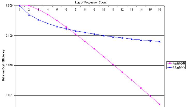
The next
graph is what I call “cost efficiency”.
It is the speed–up factor divided by the number of processors: S(N)/N. This factor measures the economic viability of the
design.
Given
the assumptions above, we see easily why large MPP designs did not appear
to be attractive in the early 1990’s and before.
The Speed–Up
Factor: S(N)
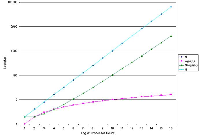
Examine a few values for the N/log2(N)
speedup: S(1024) = 102 and S(65536) = 4096.
These might be acceptable under certain specific circumstances.
The Cost
Efficiency Factor: S(N) / N
This
chart shows the real problem that was seen for MPP systems before the late
1990’s. Simply put, they were thought to
be very cost inefficient.
Linear
Speedup: The MPP Goal
The goal
of MPP system design is called “linear
speedup”, in which the performance of an N–processor system is
approximately N times that of a single processor system.
Earlier
in this lecture we made the comment that “Many important problems, particularly
ones that apply regular computations to massive data sets, are quite amenable
to parallel implementations”.
Within
the context of our lectures, the ambiguous phrase “quite amenable to parallel
implementations” acquires a specific meaning: there are well–know algorithms to
solve the problem and these algorithms can display a nearly–linear speedup when
implemented on MPP systems.
As noted
in an earlier lecture “Characteristics of Numerical Applications”, problems
that can be solved by algorithms in the class called “continuum models” are
likely to show near–linear speedup. This
is due to the limited communication between cells in the continuum grid.
There are other situations in which MPP systems might
be used. In 1990, Hennessy and Patters
on [Ref. 2, page 575] suggested that “a multiprocessor may be more effective
for a timesharing workload than a SISD [single processor]”. This seems to be the usage on the large IBM
mainframe used by CSU to teach the course in assembly language.
Linear
Speedup: The View from the Early 1990’s
Here is
what Harold Stone [Ref. 3] said in his textbook. The first thing to note is that he uses the
term “peak performance” for what we call “linear speedup”.
His
definition of peak performance is quite specific. I quote it here.
“When a multiprocessor is operating at peak
performance, all processors are engaged in useful work. No processor is idle, and no processor is
executing an instruction that would not be executed if the same algorithm were
executing on a single processor. In this
state of peak performance, all N processors are contributing to effective
performance, and the processing rate is increased by a factor of N. Peak performance is a very special state that
is rarely achievable.” [Ref. 3, page
340].
Stone
notes a number of factors that introduce inefficiencies and inhibit peak
performance. Here is his list.
1. The
delays introduced by interprocessor communication.
2. The
overhead in synchronizing the work of one processor with another.
3. The
possibility that one or more processors will run out of tasks and do nothing.
4. The
process cost of controlling the system and scheduling the tasks.
Early
History: The C.mmp
While
this lecture will focus on multicomputers, it is instructive to begin with a
review of a paper on the C.mmp, which is a shared–memory multiprocessor
developed at
The
C.mmp is described in a paper by Wulf and Harbinson [Ref. 6], which has been
noted as “one of the most thorough and balanced research–project retrospectives
… ever seen”. Remarkably, this paper
gives a thorough description of the project’s failures.
The
C.mmp is described [Ref. 6] as “a multiprocessor composed of 16 PDP–11’s, 16
independent memory banks, a crosspoint [crossbar] switch which permits any
processor to access any memory, and a typical complement of I/O
equipment”. It includes an independent
bus, called the “IP bus”, used to communicate control signals.
As of
1978, the system included the following 16 processors.
5 PDP–11/20’s, each rated at 0.20 MIPS (that
is 200,000 instructions per second)
11 PDP–11/40’s, each rated at 0.40 MIPS
3 megabytes of shared memory (650 nsec core
and 300 nsec semiconductor)
The
system was observed to compute at 6 MIPS.
The Design
Goals of the C.mmp
The goal
of the project seems to have been the construction of a simple system using as
many commercially available components as possible.
The
C.mmp was intended to be a research project not only in distributed processors,
but also in distributed software. The
native operating system designed for the C.mmp was called “Hydra”. It was intended as an OS kernel, intended to
provide only minimal services and encourage experimentation in system software.
As of
1978, the software developed on top of the Hydra kernel included file systems,
directory systems, schedulers and a number of language processors.
Another
part of the project involved the development of performance evaluation tools,
including the Hardware Monitor for recording the signals on the PDP–11 data bus
and software tools for analyzing the performance traces.
One of
the more important software tools was the Kernel Tracer, which was built into
the Hydra kernel. It allowed selected
operating system events, such as context swaps and blocking on semaphores, to
be recorded while a set of applications was running.
The Hydra kernel was originally designed based on some
common assumptions. When experimentation
showed these to be false, the Hydra kernel was redesigned.
The C.mmp:
Lessons Learned
The
researchers were able to implement the C.mmp as “a cost–effective, symmetric
multiprocessor” and distribute the Hydra kernel over all of the processors.
The use
of two variants of the PDP–11 was considered as a mistake, as it complicated
the process of making the necessary processor and operating system
modifications. The authors had used
newer variants of the PDP–11 in order to gain speed, but concluded that “It
would have been better to have had a single processor model, regardless of
speed”.
The
critical component was expected to be the crossbar switch. Experience showed the switch to be “very
reliable, and fast enough”. Early
expectations that the “raw speed” of the switch would be important were not
supported by experience.
The
authors concluded that “most applications are sped up by decomposing their
algorithms to use the multiprocessor structure, not by executing on processors
with short memory access times”.
The
simplicity of the Hydra kernel, with much system software built on top of it,
yielded benefits, such as few software errors caused by inadequate
synchronization.
The C.mmp: More
Lessons Learned
Here I
quote from Wulf & Harbison [Ref. 6], arranging their comments in an order
not found in their original. The PDP–11
was a memory–mapped architecture with a single bus, called the UNIBUS, that connected the CPU to both memory and I/O
devices.
1. “Hardware (un)reliability was our largest
day–to–day disappointment … The aggregate mean–time–between–failure (MTBF) of
C.mmp/Hydra fluctuated between two to six hours.”
2. “About two–thirds of the failures were
directly attributable to hardware problems.
There is insufficient fault detection built into the hardware.”
3. “We found the PDP–11 UNIBUS to be especially
noisy and error–prone.”
4. “The crosspoint [crossbar] switch is too
trusting of other components; it can be hung by malfunctioning memories or
processors.”
My favorite lesson learned is summarized in the
following two paragraphs in the report.
“We made a serious error in not writing good
diagnostics for the hardware. The
software developers should have written such programs for the hardware.”
“In our experience, diagnostics written by the
hardware group often did not test components under the type of load generated
by Hydra, resulting in much finger–pointing between groups.”
Task
Management in Multicomputers
The
basic idea behind both multicomputers and multiprocessors is to run multiple
tasks or multiple task threads at the same time. This goal leads to a number of requirements,
especially since it is commonly assumed that any user program will be able to
spawn a number of independently executing tasks or processes or threads.
According
to Baron and Higbie [Ref. 5], any multicomputer or multiprocessor system must
provide facilities for these five task–management capabilities.
1. Initiation A process must be able to spawn another process;
that
is, generate another process and activate it.
2. Synchronization A process must be able to suspend itself or another process
until
some sort of external synchronizing event occurs.
3. Exclusion A process must be able to monopolize a shared resource,
such
as data or code, to prevent “lost updates”.
4. Communication A process must be able to exchange messages with any
other
active process that is executing on the system.
5. Termination A process must be able to terminate itself and release
all
resources being used, without any memory leaks.
These facilities are more efficiently provided if
there is sufficient hardware support.
Hardware
Support for Multitasking
Any
processor or group of processors that supports multitasking will do so more
efficiently if the hardware provides an appropriate primitive operation.
A test–and–set operation with a binary semaphore (also called a “lock variable”) can be used for both
mutual exclusion and process synchronization.
This is best implemented as an atomic
operation, which in this context is one that cannot be interrupted until it
completes execution. It either executes
completely or fails.
The MIPS
provides another set of instructions to support synchronization. In this design, synchronization is achieved
by using a pair of instructions, issued in sequence.
After
the first instruction in the sequence is executed, the second is execute and
returns a value from which it can be deduced whether or not the instruction
pair was executed as if it were a single atomic instruction.
The MIPS
instruction pair is load linked and store conditional.
These
are often used in a spin lock
scenario, in which a processor executes in a tight loop awaiting the
availability of the shared resource that has been locked by another processor.
In fact,
this is not a necessary part of the design, but just its
most common use.
Clusters,
Grids, and the Like
There
are many applications amenable to an even looser grouping of
multicomputers. These often use
collections of commercially available computers, rather than just connecting a
number of processors together in a special network.
In the
past there have been problems of administering large clusters of computers; the
cost of administration scaling as a linear function of the number of
processors. Recent developments in
automated tools for remote management are likely to help here.
It
appears that blade servers are one
of the more recent adaptations of the cluster concept. The major advance represented by blade
servers is the ease of mounting and interconnecting the individual computers,
called “blades”, in the cluster.
In this
aspect, the blade server hearkens back to the 1970’s and the innovation in
instrumentation called “CAMAC”, which was a rack with a standard bus structure
for interconnecting instruments. This
replaced the jungle of interconnecting wires, so complex that it often took a
technician dedicated to keeping the communications intact.
Clusters
can be placed in physical proximity, as in the case of blade servers, or at
some distance and communicate via established networks, such as the
Internet. When a network is used for
communication, it is often designed using TCP/IP on top of Ethernet simply due
to the wealth of experience with this combination.
References
In this lecture, material from one or more of the
following references has been used.
1. Computer
Organization and Design, David A. Patterson & John L. Hennessy,
Morgan Kaufmann, (3rd
Edition, Revised Printing) 2007, (The course textbook)
ISBN 978 – 0 – 12 – 370606 – 5.
2. Computer
Architecture: A Quantitative Approach, John L. Hennessy and
David A. Patterson, Morgan
Kauffman, 1990. There is a later
edition.
ISBN 1 – 55860 –
069 – 8.
3. High–Performance
Computer Architecture, Harold S. Stone,
Addison–Wesley (Third Edition),
1993. ISBN 0 – 201 –
52688 – 3.
4. Structured
Computer Organization, Andrew S. Tanenbaum,
Pearson/Prentice–Hall (Fifth
Edition), 2006. ISBN 0 – 13 – 148521 – 0
5. Computer Architecture,
Robert J. Baron and Lee Higbie,
Addison–Wesley Publishing Company,
1992, ISBN 0 – 201 – 50923 – 7.
6. W. A. Wulf and S. P. Harbison, “Reflections in a pool of
processors / An
experience report on C.mmp/Hydra”,
Proceedings of the National Computer
Conference (AFIPS), June 1978.