The Cray
Series of Supercomputers
A
detailed discussion of the most significant supercomputer line of the late 20th
century.
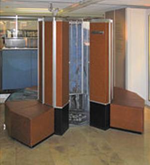
The
Cray–1 at the
Note
the design. In 1976, the magazine
Computerworld called the Cray–1
“the world’s most expensive love seat”.
History of
In
order to understand the Cray line of computers, we must look at the personal
history of Seymour Cray, the “father of the supercomputer”.
Cray
began work at Control Data Corporation soon after its founding in 1960 and
remained there until 1972. He designed
several computers, including the CDC 1604, CDC 6600, and CDC 7600. The CDC 1604 was intended just to be a good
computer; all computers beginning with the CDC 6600 were designed for speed.
The
CDC 6600 is often called the first RISC (Reduced Instruction Set Computer), due
to the simplicity of its instruction set.
The reason for its simplicity was the desire for speed.
Cray also put a lot of effort into matching the memory and I/O speed with the
CPU speed.
As he later noted, “Anyone can build a fast CPU. The trick is to build a fast system.”
The
CDC 6600 lead to the more successful CDC 7600.
Full disclosure: I have
programmed on the CDC 6600, CDC 7600, and Cray–1; I found each to be excellent.
The
CDC 8600 was to be a follow–on to the CDC 7600.
While an excellent design, it proved too complex to manufacture
successfully, and was abandoned.
Cray
left Control Data Corporation in 1972 to found Cray Research, based in
In
1989, Cray left the company in order to found Cray Computers, Inc. His reason for leaving was that he wanted to
spend more time on research, rather than just churning out the very profitable
computers that his previous company was manufacturing.
This
lead to an interesting name game:
Cray Research, Inc. producing a large number of
commercial computers
Cray Computer, Inc. mostly invested in research on future
machines.
The
Cray–3, a 16–processor system, was announced in 1993 but never delivered.
The Cray–4, a smaller version of the Cray–3 with a 1 GHz clock was ended when
the
Cray Computer Corporation went bankrupt in 1995.
Seymour
Cray died on October 5, 1996.
In
1993, Cray Research moved away from pure vector processors, producing its first
massively parallel processing (MPP) system, the Cray T3D™.
Cray
Research merged with SGI (Silicon Graphics, Inc.) in February 1996. It was spun off as a separate business unit
in August 1999. In March 2000, Cray Research was merged with Terra Computer
Company to form Cray, Inc.
Cray–1: The
Physical Machine
Here
is a schematic of the Cray–1. At the
base, it is more than 8 feet in diameter.
We may think this a large
computer, but for its time the Cray–1 was surprisingly small.
Processor
Specifications of the Cray–1
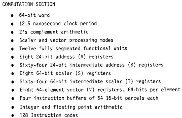
Source: Cray–1 Computer System Hardware Reference
Manual
Publication 2240004,
Revision C, November, 1977.
Memory
Specifications of the Cray–1
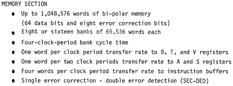
Note
that the memory size, without error correction, would be 8MB. Each word
has 64 data bits (8 bytes) as well as 8 bits for error correction.
Other
material indicates that the memory was low–order interleaved.
Source: Cray–1 Computer System Hardware Reference
Manual
Publication 2240004,
Revision C, November, 1977.
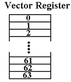
The Cray–1
Vector Registers
It
is important to understand the structure and function of the vector registers.
Each
of the vector registers is a vector of registers, best viewed as a collection
of
sixty–four registers each holding 64 bits.
A vector register held 4,096 bits.
Vector
registers are loaded from primary memory and store results back to primary
memory. One common use would be to load
a vector register from sixty–four consecutive memory words. Nonconsecutive
words could be handled if they appeared in a regular pattern, such as every
other word or every fourth word, etc.
One might consider each
register as an array, but that does not reflect its use.
The Cray–1
Vector and Scalar Registers
One
of the key design features of the Cray is the placement of a large number of
registers between the memory and the CPU units.
These function much as cache memory.
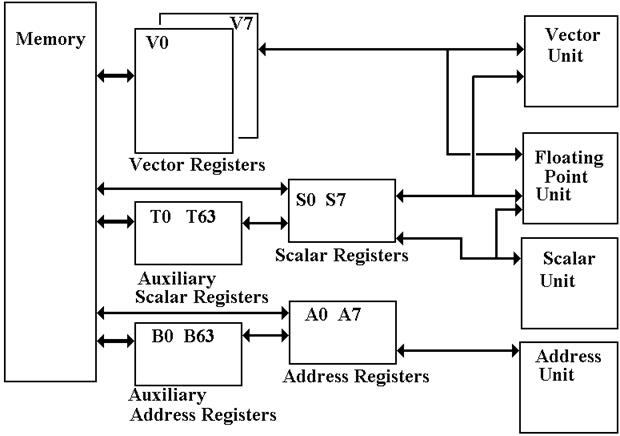
Note that the scalar and
address registers also have auxiliary registers.
Cache Memory
on the Cray
Here
we pay special attention to the Scalar Registers and the Address Registers.
All
of the registers, including the vector registers, are implemented in static
memory
with six nanosecond access time.
The
main memory has 50 nanosecond access time.
The
Cray–1 does not have explicit cache memory, but note the two pairs of register
sets.
The eight scalar registers backed up by
the sixty–three temporary registers.
The eight address registers backed up by
the sixty–three auxiliary address registers.
In
some sense, we can say that
1. the
T registers function as a cache for the S registers, and
2. the
B registers function as a cache for the A registers.
“Without the register storage
provided by the B, T, and V registers, the CRAY–1’s [memory] bandwidth of only
80 million words per second would be a serious impediment to performance.” [R.
M. Russell, 1978]
Each word is 8 bytes; 80
million words per second is 640 million bytes per second, or
one byte every 1.6 nanoseconds.
Evolution of
the Cray–1
In
this course, the main significance of the CDC 6600 and CDC 7600 computers lies
in their influence on the design of the Cray–1 and other computers in the
series.
Remember
that Seymour Cray was the principle designer of all three computers.
Here
is a comparison of the CDC 7600 and the Cray–1.
Item CDC 7600 Cray–1
Circuit Elements Discrete
Components Integrated Circuitry
Memory Magnetic
Core Semiconductor (50
nanoseconds)
Scalar (word) size 60
bits 64 bits
(plus 8 ECC bits)
Vector Registers None Eight, each
holding 64 scalars.
Scalar Registers Eight:
X0 – X7 Eight: S0 – S7
Scalar Buffer Registers None Sixty–four
T0 – T77
Octal
numbering was used.
Address Registers Eight:
A0 – A7 Eight: A0 – A7
Address Buffer Registers None Sixty–four:
B0 – B77
Two main changes: 1. Addition of the eight
vector registers.
2.
Addition of fast buffer registers for the A and S registers.
Chaining in
the Cray–1
Here
is how the technique is described in the 1978 article.
“Through a technique called
‘chaining’, the CRAY–1 vector functional units, in combination with scalar and
vector registers, generate interim results and use them again immediately
without additional memory references, which slow down the computational process
in other contemporary computer systems.”
This
is exactly the technique that we called “forwarding”
when we discussed the pipelined datapaths.
Consider
the following example using the vector multiply and vector addition operators.
MULTV V1, V2, V3 // V1[K] = V2[K] · V3[K]
ADDV V4, V1, V5 // V4[K] = V1[K] + V5[K]
Without
chaining (forwarding), the vector multiplication operation would have to finish
before the vector addition could begin.
Chaining allows a vector operation to start as soon as the individual
elements of its vector source become available.
The only restriction is that
operations being chained belong to distinct functional units, as each
functional unit can do only one thing at a time.
Vector
Startup Times
Vector
processing involves two basic steps: startup of the vector unit and pipelined
operation. As in other pipelined
designs, the maximum rate at which the vector unit executes instructions is
called the “Initiation Rate”, the
rate at which new vector operations are initiated when the vector unit is
running at “full speed”.
The
initiation rate is often expressed as a time, so that a vector unit that
operated at
100 million operations per second would have an initiation rate of 10
nanoseconds.
I
know: rates are not times. This is just
the common terminology.
The
time to process a vector depends on the length of the vector. For a vector with
length N (containing N elements) we have
T(N) = Start–Up_Time +
The
time per result is then T = (Start–Up Time) / N + Initiation_Rate.
For
short vectors (small values of N), this time may exceed the initiation rate of
the scalar execution unit. An important
measure of the balance of the design is the vector size at which the vector
unit can process faster than the scalar unit.
For a Cray–1, this crossover
size was between 2 and 4; 2 £ N £ 4.
For N > 4, the vector unit was always faster.
Experimental
Results: Scalar/Vector Timing
Here
are some comparative data for mathematical operations (Log, cosine, square
root, and exponential), showing the per–result times as a function of vector
length. Note the low crossover point,
for vectors larger than N = 5, the vector unit is much faster.
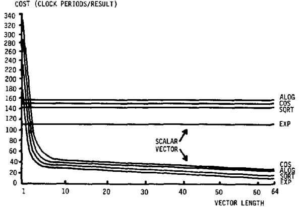
The time cost is given in
clock ticks, not nanoseconds. See
Russell, 1978.
The Cray
X–MP and Cray Y–MP
The
fundamental tension at Cray Research, Inc. was between Seymour Cray’s desire to
develop new and more powerful computers and the need to keep the cash flow
going.
Seymour
Cray realized the need for a cash flow at the start. As a result, he decided not to pursue his
ideas based on the CDC 8600 design and chose to develop a less aggressive
machine. The result was the Cray–1,
which was still a remarkable machine.
With its cash flow insured, the company then organized
its efforts into two lines of work.
1. Research and development on the CDC 8600
follow–on, to be called the Cray–2.
2. Production of a line of computers that were
derivatives of the Cray–1 with
improved technologies. These were called the X–MP, Y–MP, etc.
The X–MP was introduced in 1982. It was a dual–processor computer with a 9.5
nanosecond (105 MHz) clock and 16 to 128 megawords of static RAM main memory.
A four–processor model was introduced in 1984 with a 8.5 nanosecond clock.
The Y–MP was introduced in 1988, with up to eight
processors that used VLSI chips.
It had a 32–bit address space, with up to 64 megawords of static RAM main
memory.
The Y–MP M90, introduced in 1992, was a large–memory
variant of the Y–MP that replaced the static RAM memory with up to 4 gigawords
of DRAM.
The Cray–2
While
his assistant, Steve Chen, oversaw the production of the commercially
successful X–MP and Y–MP series, Seymour Cray pursued his development of the
Cray–2, a design based on the CDC 8600, which Cray had started while at the
Control Data Corporation.
The
original intent was to build the VLSI chips from gallium arsenide (GaAs), which
would allow must faster circuitry. The
technology for manufacturing GaAs chips was not then mature enough to be useful
as circuit elements in a large computer.
The
Cray–2 was a four–processor computer that had 64 to 512 megawords of 128–way
interleaved DRAM memory. The computer
was built very small in order to be very fast, as a result the circuit boards
were built as very compact stacked cards.
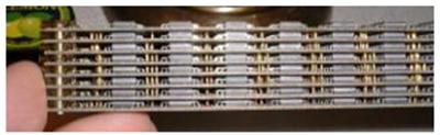
Due
to the card density, it was not possible to use air cooling. The entire system was immersed in a tank of
Fluorinert™, an inert liquid intended to be a blood substitute.
When introduced in 1985, the
Cray–2 was not significantly faster than the Y–MP. It sold only thirty copies, all to customers
needing its large main memory capacity.
The Cray–3
and the End of an Era
After the Cray–2, Seymour Cray began another very
aggressive design: the Cray–3.
This was to be a very small computer that fit into a cube one foot on a side.
Such a design would require retention of the
Fluorinert cooling system. It would also
be very difficult to manufacture as it would require robotic assembly and
precision welding. It would also have
been very difficult to test, as there was no direct access to the internal
parts of the machine.
The Cray–3 had a 2 nanosecond cycle time (500
MHz). A single processor machine would
have a performance of 948 megaflops; the 16–processor model would have operated
at 15.2 gigaflops. The 16–unit model was
never built.
The Cray–3 was delivered in 1993. In 1994, Cray Research, Inc. released the T90
with a 2.2 nanosecond clock time and eight times the performance of the Cray–3.
In
the end, the development of traditional supercomputers ran into several
problems.
1. The end of the cold war reduced the pressing
need for massive computing facilities.
2. The rise of microprocessor technology allowing
much faster and cheaper processors.
3. The rise of VLSI technology, making multiple
processor systems more feasible.
Supercomputers
vs. Multiprocessor Clusters
“If you were plowing a field,
which would you rather use: Two strong
oxen or 1024 chickens”.
Although
Seymour Cray said it more colorfully, there were many objections to the
transition from the traditional vector supercomputer (with a few processors) to
the massively parallel computing that replaced it.
This
slide quotes from an overview article written in 1984. It assessed the commercial viability of
traditional vector processors and multiprocessor systems.
The
key issue in assessing the commercial viability of a multiple–processor system
is the speedup factor; how much
faster is a processor with N processors.
Here are two opinions from the 1984 IEEE tutorial on supercomputers.
“The speedup factor of using
an n–processor system over a
uniprocessor system has been theoretically estimated to be within the range
(log2n, n/log2n). For example, the speedup
range is less than 6.9 for n =
16. Most of today’s commercial
multiprocessors have only 2 to 4 processors in a system.”
“By the late 1980s, we may
expect systems of 8–16 processors.
Unless the technology changes drastically, we will not anticipate
massive multiprocessor systems until the 90s.”
As we shall see soon,
technology has changed drastically.
The Cray XT–5
Here
is a picture of the Cray XT–5, one of the later and faster products from Cray,
Inc.
It is a MPP (Massively Parallel Processor) system, launched in November 2007.
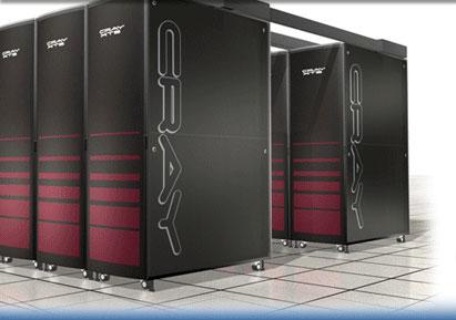
This
is built from a number of Quad–Core AMD Opteron™ processor cores.
The
Operating System is a variant of Linux.
References:
Wikipedia: http://en.wikipedia.org/wiki/Cray-1
http://en.wikipedia.org/wiki/Cray_X-MP
The
History of Computing Project http://www.thocp.net/hardware/cray_1.htm
Cray,
Inc. http://www.cray.com/
R.
M. Russell, “The Cray–1 computer system.”, Communications of the ACM,
21(1):63–72, 1978.
Kai
Hwang, “Evolution of Modern Supercomputers”, the introduction to Chapter 1 in
the IEEE Tutorial Supercomputers: Design
and Applications, 1984.
ISBN 0 – 8186 – 0581 – 2.