Assessing and Understanding Performance

This set of slides is based on Chapter 4, Assessing and Understanding Performance, of the book Computer Organization and Design by Patterson and Hennessy.

Here are some typical comments.

1. I want a better computer.

2. I want a faster computer.

3. I want a computer or network of computers that does more work.

4. I have the latest game in “World of Warcraft” and want a computer that can play it.

QUESTION: What does “better” mean?

What does “faster” really mean, beyond its obvious meaning?

What does it mean for a computer or network to do more work?

COMMENT: The last requirement is quite easy to assess if you have a copy of the
game. Just play the game on a computer of that model and see if
you get performance that is acceptable. Are the graphics realistic?

The reference to the gaming world brings home a point on performance.
In games one needs both a fast computer and a great graphics card.
It is the performance of the entire system that matters.

The Need for Greater Performance

Aside from the obvious need to run games with more complex plots and more detailed and realistic graphics, are there any other reasons to desire greater performance?

We shall study supercomputers later. At one time supercomputers, such as the Cray 2 and the CDC Cyber 205, were the fastest computers on the planet.

One distinguished computer scientist gave the following definition of a supercomputer.
“It is a computer that is only one generation behind the computational needs of the day.”

What applications require such computational power?

1. Weather modeling. We would like to have weather predictions that are accurate
up to two weeks after the prediction. This requires a great deal of computational
power. It was not until the 1990’s that the models had the Appalachian Mountains.

2. We would like to model the flight characteristics of an airplane design before we
actually build it. We have a set of equations for the flow of air over the wings and
fuselage of an aircraft and we know these produce accurate results.

The only problem here is that simulations using these exact equations would take
hundreds of years for a typical airplane. Hence we run approximate solutions and
hope for faster computers that allow us to run less–approximate solutions.

The Job Mix

The World of Warcraft example above is a good illustration of a job mix. Here the job mix is simple; just one job – run this game.

This illustrates the very simple statement “The computer that runs your job fastest is the one that runs your job fastest”. In other words, measure its performance on your job.

Most computers run a mix of jobs; this is especially true for computers owned by a company or research lab, which service a number of users. In order to assess the suitability of a computer for such an environment, one needs a proper “job mix”, which is a set of computer programs that represent the computing need of one’s organization.

Your instructor once worked at Harvard College Observatory. The system administrator for our computer lab spent considerable effort in selecting a proper job mix, with which he intended to test computers that were candidates for replacing the existing one.

This process involved detailed discussions with a large number of users, who (being physicists and astronomers) all assumed that they knew more about computers than he did. Remember that in the 1970’s; this purchase was for a few hundred thousand dollars.

These days, few organizations have the time to specify a good job mix. The more common option is to use the results of commonly available benchmarks, which are
job mixes tailored to common applications.

What Is Performance?

Here we make the observation that the terms “high performance” and “fast” have various meanings, depending on the context in which the computer is used.

In many applications, especially the old “batch mode” computing, the measure was the number of jobs per unit time. The more user jobs that could be processed; the better.

For a single computer running spreadsheets, the speed might be measured in
the number of calculations per second.

For computers that support process monitoring, the requirement is that the computer correctly assesses the process and takes corrective action (possibly to include warning a human operator) within the shortest possible time.

Some systems, called “hard real time”, are those in which there is a fixed time interval during which the computer must produce and answer or take corrective action. Examples of this are patient monitoring systems in hospitals and process controls in oil refineries.

As an example, consider a process monitoring computer with a required response time
of 15 seconds. There are two performance measures of interest.

1. Can it respond within the required 15 seconds? If not, it cannot be used.

2. How many processes can be monitored while guaranteeing the required 15 second
response time for each process being monitored. The more, the better.

The Average (Mean) and Median

In assessing performance, we often use one or more tools of arithmetic.
We discuss these here.

The problem starts with a list of N numbers (A₁, A₂, …, A_N), with N ³ 2.

For these problems, we shall assume that all are positive numbers: A_J > 0, 1 £ J £ N.

Arithmetic Mean and Median
The most basic measures are the average (mean) and the median.

The average is computed by the formula (A₁ + A₂ + + A_N) / N.

The median is the “value in the middle”. Half of the values are larger and half are
smaller. For a small even number of values, there might be two candidate median values.

For most distributions, the mean and the median are fairly close together. However, the two values can be wildly different.

For example, there is a high–school class in the state of Washington in which the average income of its 100 members is about $1,500,000 per year; that’s a lot of money.

If the salary of Bill Gates and one of his cohorts at Microsoft are removed, the average
becomes about $50,000. This value is much closer to the median.

Disclaimer: This example is from memory, so the numbers are not exact.

Weighted Averages,

In certain averages, one might want to pay more attention to some values than others.
For example, in assessing an instruction mix, one might want to give a weight to each instruction that corresponds to its percentage in the mix.

Each of our numbers (A₁, A₂, …, A_N), with N ³ 2, has an associated weight.
So we have (A₁, A₂, …, A_N) and (W₁, W₂, …, W_N). The weighted average is given by the formula (W₁·A₁ + W₂·A₂ …+ W_N·A_N) / (W₁ + W₂ +…+ W_N).

NOTE: If all the weights are equal, this value becomes the arithmetic mean.

Consider the table adapted from our discussion of RISC computers.

Language	Pascal	FORTRAN	Pascal	C	SAL	Average
Workload	Scientific	Student	System	System	System
Assignment	74	67	45	38	42	53.2
Loop	4	3	5	3	4	3.8
Call	1	3	15	12	12	8.6
If	20	11	29	43	36	27.8
GOTO	2	9	--	3	--	4.7

The weighted average 0.532·T_A + 0.038·T_L + 0.086·T_C + 0.278·T_I + 0.047·T_G to assess an ISA (Instruction Set Architecture) to support this job mix.

The Geometric Mean and the Harmonic Mean

Geometric Mean

The geometric mean is the Nth root of the product (A₁·A₂·…·A_N)^1/N.
It is generally applied only to positive numbers, as we are considering here.

Some of the SPEC benchmarks (discussed later) report the geometric mean.

Harmonic Mean

The harmonic mean is N / ( (1/A₁) + (1 / A₂) + … + ( 1 / A_N) )

This is more useful for averaging rates or speeds. As an example, suppose that you drive at 40 miles per hour for half the distance and 60 miles per hour for the other half.
Your average speed is 48 miles per hour.

If you drive 40 mph for half the time and 60 mph for half the time, the average is 50.

Example:

Drive 300 miles at 40 mph. The time taken is 7.5 hours.

Drive 300 miles at 60 mph. The time taken is 5.0 hours.

You have covered 600 miles in 12.5 hours, for an average speed of 48 mph.

But: Drive 1 hour at 40 mph. You cover 40 miles
Drive 1 hour at 60 mph. You cover 60 miles. That is 100 miles in 2 hours; 50 mph.

Measuring Execution Time

Whatever it is, performance is inversely related to execution time. The longer the execution time, the less the performance.

Again, we assess a computer’s performance by measuring the time to execute either a single program or a mix of computer programs, the “job mix”, that represents the computing work done at a particular location.

For a given computer X, let P(X) be the performance measure, and
E(X) be the execution time measure.

What we have is P(X) = K / E(X), for some constant K. The book has K = 1.

This raises the question of how to measure the execution time of a program.

Wall–clock time: Start the program and note the time on the clock.
When the program ends, again note the time on the clock.
The difference is the execution time.

This is the easiest to measure, but the time measured may include time that the processor spends on other users’ programs (it is time–shared), on operating system functions, and similar tasks. Nevertheless, it can be a useful measure.

Some people prefer to measure the CPU Execution Time, which is the time the CPU spends on the single program. This is often difficult to estimate based on clock time.

Reporting Performance: MIPS, MFLOPS, etc.

While we shall focus on the use of benchmark results to report computer performance, we should note that there are a number of other measures that have been used.

The first is MIPS (Million Instructions Per Second).

Another measure is the FLOPS sequence, commonly used to specify the performance of supercomputers, which tend to use floating–point math fairly heavily. The sequence is:

MFLOPS Million Floating Point Operations Per Second

GFLOPS Billion Floating Point Operations Per Second
(The term “giga” is the standard prefix for 10⁹.)

TFLOPS Trillion Floating Point Operations Per Second
(The term “tera” is the standard prefix for 10¹².)

The reason we do not have “BLOPS” is a difference in the usage of the word “billion”. In American English, the term “billion” indicates “one thousand million”. In some European countries the term “billion” indicates “one million million”.

This was first seen in the high energy physics community, where the unit of measure
“BeV” was replaced by “GeV”, but not before the Bevatron was named.

I leave it to the reader to contemplate why the measure “MIPS” was not extended to
either “BIPS” or “GIPS”, much less “TIPS”.

Using MIPS as a Performance Measure

There are a number of reasons why this measure has fallen out of favor.

One of the main reasons is that the term “MIPS” had its origin in the marketing departments of IBM and DEC, to sell the IBM 370/158 and VAX–11/780.

One wag has suggested that the term “MIPS” stands for
“Meaningless Indicator of Performance for Salesmen”.

A more significant reason for the decline in the popularity of the term “MIPS” is the fact that it just measures the number of instructions executed and not what these do.

Part of the RISC movement was to simplify the instruction set so that instructions could be executed at a higher clock rate. As a result these instructions are less complex and do less than equivalent instructions in a more complex instruction set.

For example, consider the instruction A[K++] = B as part of a loop. The VAX supports an auto–increment mode, which uses a single instruction to store the value into the array and increment the index. Most RISC designs require two instructions to do this.

Put another way, in order to do an equivalent amount of work a RISC machine must run at a higher MIPS rating than a CISC machine.

HOWEVER: The measure does have merit when comparing two computers with
identical organization.

GFLOPS, TFLOPS, and PFLOPS

The term “PFLOP” stands for “PetaFLOP” or 10¹⁵ floating–point operations per second.
This is the next goal for the supercomputer community.

The supercomputer community prefers this measure, due mostly to the great importance of floating–point calculations in their applications. A typical large–scale simulation may devote 70% to 90% of its resources to floating–point calculations.

The supercomputer community has spent quite some time in an attempt to give a precise definition to the term “floating point operation”. As an example, consider the following code fragment, which is written in a standard variety of the FORTRAN language.

DO 200 J = 1, 10

200 C(J) = A(J)*B(J) + X

The standard argument is that the loop represents only two floating–point operations: the multiplication and the addition. I can see the logic, but have no other comment.

The main result of this measurement scheme is that it will be difficult to compare the performance of the historic supercomputers, such as the CDC Cyber 205 and the Cray 2, to the performance of the modern day “champs” such as a 4 GHz Pentium 4.

In another lecture we shall investigate another use of the term “flop” in describing the classical supercomputers, when we ask “What happened to the Cray 3?”

CPU Performance and Its Factors

The CPU clock cycle time is possibly the most important factor in determining
the performance of the CPU. If the clock rate can be increased, the CPU is faster.

In modern computers, the clock cycle time is specified indirectly by specifying the clock cycle rate. Common clock rates (speeds) today include 2GHz, 2.5GHz, and 3.2 GHz.

The clock cycle times, when given, need to be quoted in picoseconds, where
1 picosecond = 10^–12 second; 1 nanosecond = 1000 picoseconds.

The following table gives approximate conversions between clock rates and clock times.

Rate Clock Time

1 GHz 1 nanosecond = 1000 picoseconds

2 GHz 0.5 nanosecond = 500 picoseconds

2.5 GHz 0.4 nanosecond = 400 picoseconds

3.2 GHz 0.3125 nanosecond = 312.5 picoseconds

We shall return later to factors that determine the clock rate in a modern CPU.

There is much more to the decision than “crank up the clock rate until the CPU
fails and then back it off a bit”.

CPI: Clock Cycles per Instruction

This is the number of clock cycles, on average, that the CPU requires to execute an instruction. We shall later see a revision to this definition.

Consider the Boz–5 design used in my offerings of CPSC 5155. Each instruction would take either 1, 2, or 3 major cycles to execute: 4, 8, or 12 clock cycles.

In the Boz–5, the instructions referencing memory could take either 8 or 12 clock cycles,
those that did not reference memory took 4 clock cycles.

A typical Boz–5 instruction mix might have 33% memory references, of which 25% would involve indirect references (requiring all 12 clock cycles).

The CPI for this mix is CPI = (2/3)·4 + 1/3·(3/4·8 + 1/4·12)
= (2/3)·4 + 1/3·(6 + 3)
= 8/3 + 3 = 17/3 = 5.33.

The Boz–5 has such a high CPI because it is a traditional fetch–execute design. Each instruction is first fetched and then executed. Adding a prefetch unit on the Boz–5 would allow the next instruction to be fetched while the present one is being executed. This removes the three clock cycle penalty for instruction fetch, so that the number of clock cycles per instruction may now be either 1, 5, or 9.

For this CPI = (2/3)·1 + 1/3·(3/4·5 + 1/4·9) = 2/3 + 1/3·(15/4· + 9/4)
= 2/3 + 1/3·(24/4) = 2/3 + 1/3·6 = 2.67. This is still slow.

A Preview on the RISC Design Problem

We shall discuss this later, but might as well bring it up now.

The RISC designs focus on lowering the CPI, with the goal of
one clock cycle per instruction.

There are two measures that must be considered here.

(Clock cycles per instruction)·(Clock cycle time), and

(Assembly language instructions per high–level instruction)·
(Clock cycles per instruction)·(Clock cycle time).

The second measure is quite important. It is common for the CISC designs (those, such as the VAX, that are not RISC) to do poorly on the first measure, but well on the second as each high level language statement generates fewer assembly language statements.

The textbook’s measure that is equivalent to this second measure is
(Instruction count)·(CPI)·(Clock cycle time).
This really focuses on the same issue as my version of the measure.

NOTE: More from the comedy department.
Some wags label the computers of the VAX design line as “VAXen”.
We get our laughs where we can find them.

More on Benchmarks

As noted above, the best benchmark for a particular user is that user’s job mix.

Only a few users have the resources to run their own benchmarks on a number
of candidate computers. This task is now left to larger test labs.

These test labs have evolved a number of synthetic benchmarks to handle the tests.
These benchmarks are job mixes intended to be representative of real job mixes.
They are called “synthetic” because they usually do not represent an actual workload.

The Whetstone benchmark was first published in 1976 by Harold J. Curnow and Brian A. Wichman of the British National Physical Laboratory. It is a set of floating–point intensive applications with many calls to library routines for computing trigonometric and exponential functions. Supposedly, it represents a scientific work load.

Results of this are reported either as
KWIPS (Thousand Whetstone Instructions per Second), or
MWIPS (Million Whetstone Instructions per Second)

The Linpack (Linear Algebra Package) benchmark is a collection of subroutines to
solve linear equations using double–precision floating–point arithmetic. It was published in 1984 by a group from Argonne National Laboratory. Originally in FORTRAN 77, it has been rewritten in both C and Java. These results are reported in FLOPS:
GFLOPS, TFLOPS, etc. (See a previous slide.)

Games People Play (with Benchmarks)

Synthetic benchmarks (Whetstone, Linpack, and Dhrystone) are convenient, but easy to fool. These problems arise directly from the commercial pressures to quote
good benchmark numbers in advertising copy. This problem is seen in two areas.

1. Manufacturers can equip their compilers with special switches to emit code that is
tailored to optimize a given benchmark at the cost of slower performance on a more
general job mix. “Just get us some good numbers!”

2. The benchmarks are usually small enough to be run out of cache memory.
This says nothing of the efficiency of the entire memory system, which must
include cache memory, main memory, and support for virtual memory.

Our textbook mentions the 1995 Intel special compiler that was designed only to excel in the SPEC integer benchmark. Its code was fast, but incorrect.

Bottom Line: Small benchmarks invite companies to fudge their results.
Of course they would say “present our products in the best light.”

More Games People Play (with Benchmarks)

Your instructor recalls a similar event in the world of Lisp machines. These were specialized workstations designed to optimize the execution of the LISP language widely used in artificial intelligence applications.

The two “big dogs” in this arena were Symbolics and LMI (Lisp Machines Incorporated).
Each of these companies produced a high–performance Lisp machine based on a microcoded control unit. These were the Symbolics–3670 and the LMI–1.

Each company submitted its product for testing by a graduate student who was writing
his Ph.D. dissertation on benchmarking Lisp machines.

Between the time of the first test and the first report at formal conference, LMI customized its microcode for efficient operation on the benchmark code.

At the original test, the LMI–1 had only 50% of the performance of the Symbolics–3670. By the time of the conference, the LMI–1 was now “officially” 10% faster.

The managers from Symbolics, Inc. complained loudly that the new results were meaningless. However, these complaints were not necessary as every attendee at the conference knew what had happened and acknowledged the Symbolics–3670 as faster.

NOTE: Neither design survived the Intel 80386, which was much cheaper
than the specialized machines, had an equivalent GUI, and was much cheaper.

At the time, the costs were about $6,000 vs. about $100,000.

The SPEC Benchmarks

The SPEC (Standard Performance Evaluation Corporation) was founded in 1988 by a consortium of computer manufacturers in cooperation with the publisher of the trade magazine The Electrical Engineering Times. (See www.spec.org)

As of 2007, the current SPEC benchmarks were:

1. CPU2006 measures CPU throughput, cache and memory access speed,
and compiler efficiency. This has two components:

SPECint2006 to test integer processing, and
SPECfp2006 to test floating point processing.

2. SPEC MPI 2007 measures the performance of parallel computing systems and clusters
running MPI (Message–Passing Interface) applications.

3. SPECweb2005 a set of benchmarks for web servers, using both HTTP and HTTPS.

4. SPEC JBB2005 a set of benchmarks for server–side Java performance.

5. SPEC JVM98 a set of benchmarks for client–side Java performance.

6. SPEC MAIL 2001 a set of benchmarks for mail servers.

The student should check the SPEC website for a listing of more benchmarks.

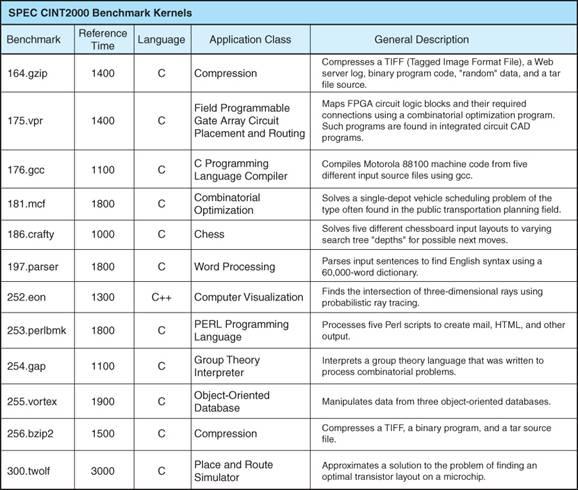
The SPEC CINT2000 Benchmark Suite

The CINT2000 is an earlier integer benchmark suite. It evolved into SPECint2006.
Here is a listing of its main components.

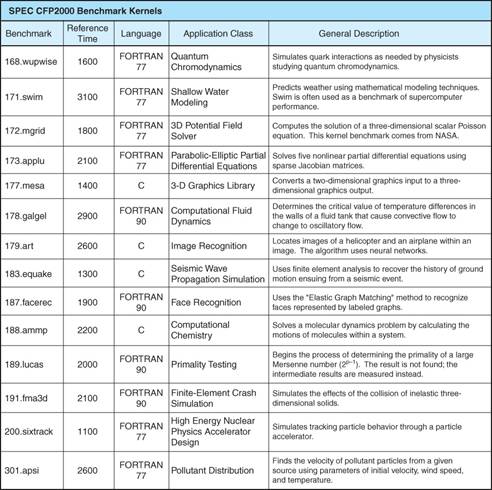
The SPEC CFP2000 Benchmark Suite

The CFP2000 is an earlier integer benchmark suite. It evolved into SPECfp2006.
Here is a listing of its main components.

Some Concluding Remarks on Benchmarks

First, remember the great temptation to manipulate benchmark results for
commercial advantage. As the Romans said, “Caveat emptor”.

Also remember to read the benchmark results skeptically and choose the
benchmark that most closely resembles your own workload.

Finally, do not forget Amdahl’s Law, which computes the improvement in overall system performance due to the improvement in a specific component.

This law was formulated by George Amdahl in 1967. One formulation of the law
is given in the following equation.

S = 1 / [ (1 – f) + (f /k) ]

where S is the speedup of the overall system,

f is the fraction of work performed by the faster component, and

k is the speedup of the new component.

It is important to note that as the new component becomes arbitrarily fast (k ® ¥),
the speedup approaches the limit S_¥ = 1/(1 – f).

If the newer and faster component does only 50% of the work, the maximum speedup is 2. The system will never exceed being twice as fast due to this modification.