Pipelining the CPU

There are two types of simple control unit design:

1. The single–cycle CPU with its slow clock, which executes
one instruction per clock pulse.

2. The multi–cycle CPU with its faster clock. This divides the execution
of an instruction into 3, 4, or 5 phases, but takes that number of clock
pulses to execute a single instruction.

We now move to the more sophisticated CPU design that allows the apparent
execution of one instruction per clock cycle, even with the faster clock.

This design technique is called pipelining, though it might better be considered
as an assembly line.

In this discussion, we must focus on throughput as opposed to the time to execute
any single instruction. In the MIPS pipeline we consider, each instruction will take
five clock pulses to execute, but one instruction is completed every clock pulse.

The measure will be the number of instructions executed per second, not the time
required to execute any one instruction. This measure is crude; more is better.

The Assembly Line

Here is a picture of the Ford assembly line in 1913.

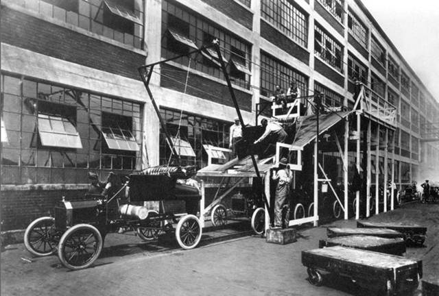
It is the number of cars per hour that roll off the assembly line that is important,
not the amount of time taken to produce any one car.

More on the Automobile Assembly Line

Henry Ford began working on the assembly line concept about 1908 and had essentially
perfected the idea by 1913. His motivations are worth study.

In previous years, automobile manufacture was done by highly skilled technicians, each
of whom assembled the whole car.

It occurred to Mr. Ford that he could get more get more workers if he did not require such
a high skill level. One way to do this was to have each worker perform only a small
number of tasks related to manufacture of the entire automobile.

It soon became obvious that is was easier to bring the automobile to the worker than have
the worker (and his tools) move to the automobile. The assembly line was born.

The CPU pipeline has a number of similarities.

1. The execution of an instruction is broken into a number of simple steps, each
of which can be handled by an efficient execution unit.

2. The CPU is designed so that it can simultaneously be executing a number of
instructions, each in its own distinct phase of execution.

3. The important number is the number of instructions completed per unit time,
or equivalently the instruction issue rate.

An Obvious Constraint on Pipeline Designs

This is mentioned, because it is often very helpful to state the obvious.

In a stored program computer, instruction execution is essentially sequential,
with occasional exceptions for branches and jumps.

In particular, the effect of executing a sequence of instructions must be as
if they had been executed in the precise order in which they were written.

Consider the following code fragment.

add $s0, $t0, $t1 # $s0 = $t0 + $t1

sub $t2, $s0, $t3 # $t2 = $s0 - $t3
# Must use the updated value of $s0

This does not have the same effect as it would if reordered.

sub $t2, $s0, $t3 # $t2 = $s0 - $t3

add $s0, $t0, $t1 # $s0 = $t0 + $t1

In particular, the first sequence of instructions demands that the value of register $s0
be updated before it is used in the subtract instruction. As we shall see, this places a
constraint on the design of any pipelined CPU.

Issue Rate vs. Time to Complete Each Instruction

Here the laundry analogy in the textbook can be useful.

The time to complete a single load in this model is two hours, start to finish.

In the “pipelined variant”, the issue rate is one load per 30 minutes; a fresh
load goes into the washer every 30 minutes.

After the “pipeline is filled” (each stage is functioning), the issue rate
is the same as the completion rate.

Our example breaks the laundry processing into four natural steps. As with CPU
design, it is better to break the process into steps with logical foundation.

In all pipelined (assembly lined) processes, it is better if each step takes about
the same amount of time to complete. If one step takes excessively long to
complete, we can allocate more resources to it.

This observation leads to the superscalar design technique, to be discussed later.

The Earliest Pipelines

The first problem to be attacked in the development of pipelined architectures was
the fetch–execute cycle.

The instruction is fetched and then executed.

How about fetching one instruction while a previous instruction is executing?
This would certainly speed things up a bit.

It is here that we see one of the advantages of RISC designs, such as the MIPS.

Each instruction has the same length (32 bits) as any other instruction, so that an
instruction can be prefetched without taking time to identify it.

Remember that, with the Pentium 4, the IA–32 architecture is moving toward translation
of the machine language instructions into much simpler micro–operations stored in a
trace buffer. These can be prefetched easily as they have constant length.

Instruction–Level Parallelism: Instruction Prefetch

Break up the fetch–execute cycle and do the two in parallel.

This dates to the IBM Stretch (1959)

The prefetch buffer is implemented in the CPU with on–chip registers.

The prefetch buffer is implemented as a single register or a queue.
The CDC–6600 buffer had a queue of length 8.

Think of the prefetch buffer as containing the IR (Instruction Register)

When the execution of one instruction completes, the next one is already
in the buffer and does not need to be fetched.

Any program branch (loop structure, conditional branch, etc.) will invalidate the contents
of the prefetch buffer, which must be reloaded.

The MIPS Pipeline

The MIPS pipeline design is based on the five–step instruction execution discussed in
the previous chapter. The pipeline will have five stages.

MIPS instructions are executed in five steps:

1. Fetch instruction from memory.

2. Decode the instruction and read two registers.

3. Execute the operation or calculate an address.

4. Access an operand in data memory or write back a result.

5. For LW only, write the results of the memory read into a register.

The pipeline design calls for a five–stage pipeline, with one stage for
each step in the execution of a typical instruction.

The clock rate will be set by the slowest execution step, as the pipeline will
have a number of instructions in different phases during any one clock cycle.

As we shall see later, the MIPS instruction set is particularly designed for efficient
execution in a pipelined CPU.

Pipelining and the Split Cache

Almost all modern computers with cache memory use a split level–1 cache.

One reason for this is that the design supports the pipelined CPU.

The I–Cache and D–Cache are independent memories. The IF pipeline stage can
access the I–Cache on every clock pulse without interfering with access to the
D–Cache by the MEM and WB stages.

The MIPS Single–Cycle Datapath

Figure 4.33 shows the single–cycle datapath, divided into five sections. One section is
associated with each step in the five step processing. We shall say more on this later.

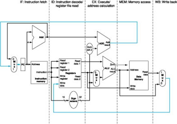
Think of instructions as “flowing left to right”.

Setting the Clock Rate for Pipelining

In a pipelined CPU, the execution is broken into a number of steps.

In a simple pipeline, each step is allocated the same amount of time.

Figure 4.26 from the textbook shows some timings used to set a clock rate.

Instruction Class	Instruction Fetch	Register Read	ALU Operation	Data Access	Register Write	Total Time
LW	200 ps	100 ps	200 ps	200 ps	100 ps	800 ps
SW	200 ps	100 ps	200 ps	200 ps		700 ps
RR Format	200 ps	100 ps	200 ps		100 ps	600 ps
BEQ	200 ps	200 ps	200 ps			500 ps

In a pipeline, the goal is for each stage to work on part of an instruction
at every clock cycle.

Here, the clock rate cannot exceed 5 GHz (200 ps per clock pulse) so that the slower
operations can complete during the time allotted.

Recall that present heat–removal technology limits the clock rate to something
less than 4 GHz.

Designing Instruction Sets (and Compilers) for Pipelining

As a design feature, pipelining is similar to very many enhancements. If added “after
the fact”, it will be very hard to implement correctly.

It is much better to design the ISA (Instruction Set Architecture) with pipelining in mind.
This brings home a very important feature of design: the compilers, operating system,
ISA, and hardware implementation must all be designed at the same time.

Put another way, the system must be designed as a whole, with appropriate trade–offs
between subsystems in order to optimize the overall performance.

Features of the MIPS design that were intended to facilitate pipelining include:

1. The fact that all instructions are the same length.

2. The small number of instruction formats.

3. The regularity of the instruction format, always beginning with a 6–bit opcode,
followed by two 5–bit register identifiers.

4. The use of the load/store design, restricting memory accesses to
only two, well defined, steps.

5. The fact that only one instruction writes to memory, and that as the
last stage in instruction execution.

6. The fact that all instructions are aligned on addresses that are a multiple of four.

The Pipeline: Ideals and Hazards

Ideally a pipelined CPU should function in much the same way as an automobile
assembly line, each stage operates in complete independence of every other stage.

The instruction is issued and enters the pipeline. Ideally, as it progresses through the
pipeline it does not depend on the results of any other instruction now in the pipeline.

Obviously, this cannot be the case. What we can say is the following.

1. It is not possible for any instruction to depend on the results of instructions
that will execute in the future. This is a logical impossibility.

2. Instructions can have dependence only on those previously executed; however,
there are no issues associated with dependence on instructions
that have completed execution and exited the pipeline.

3. It is possible, and practical, to design a compiler that will minimize problems
in the pipeline. This is a desirable result of the joint design of compile and ISA.

4. It is not possible for the compiler to eliminate all pipelining problems without
reducing the CPU to a non–pipelined datapath, which is unacceptably slow.

These pipeline problems are called hazards. They come in three varieties:
structural hazards, data hazards, and control hazards.

Ideal Pipeline Execution

Ideally a new instruction is issued on every clock cycle and, after the pipeline is filled,
an instruction is completed on every clock cycle.

In our example, we assume a 5 GHz clock, with a clock pulse time of 200 picoseconds.

We use the above graphical representation to show three instructions as each passes
through all steps of the CPU datapath.

Pipeline Hazards

A pipeline hazard occurs when an instruction cannot complete a step in its execution,
due to some event in the previous clock cycle.

When an instruction must be held for one or more clock pulses in order to complete
a step in its execution, this is called a “pipeline stall”, informally a “bubble”.

The three types of hazards are as follows.

Structural hazards occur when the instruction set architecture does not match the design
of the control unit. The hardware cannot support the combination of instructions that we
want to execute in the same clock cycle. The MIPS is designed to avoid this type.

Data hazards are due to tight dependencies in sequences of machine language
instructions. These occur when one step in the pipeline must await the completion of a
previous instruction. A good compiler can reduce these hazards, but not eliminate them.

Control hazards, also called branch hazards, arise from the need to make a decision
based on the results of one instruction while others are executing. A typical example
would be the execution of a conditional branch instruction. If the branch is taken, the
instructions currently in the pipeline might be invalid.

Data Hazards

A data hazard is an occurrence in which a planned instruction cannot execute in the
proper clock cycle due to dependence on an earlier instruction still in the pipeline.

Example: Suppose the following sequence of two instructions.

add $s0, $t0, $t1 # $s0 = $t0 + $t1

sub $t2, $s0, $t3 # $t2 = $s0 - $t3
# Must use the updated value of $s0

Consider the following sequence events, with a time line labeled by clock pulses.

T0: The add instruction is fetched

T1: The add instruction is decoded and registers $t0 and $t1 read
The sub instruction is fetched.

T2: The addition is performed in the ALU.
The sub instruction is decoded.
The attempt to read $s0 yields a data hazard. At this point, the
results of the addition have yet to be written back to $s0.

This situation can result in a stall for a number of clock cycles.

The “Three Bubble Solution”

Without modification to the CPU, the Instruction Decode/Register Read stage of the
instruction cannot proceed until the add instruction has written back to the register file.

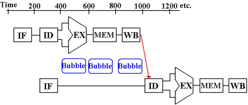
Note that the subtract instruction is stalled for three clock cycle (hence three “bubbles”)
until the updated value of $s0 can be read from the register file.

Again, a clever compiler can somewhat reduce the occurrences of data hazards,
but it cannot eliminate them entirely. The CPU must handle some.

Forwarding or Bypassing

Consider again the following sequence of two instructions.

add $s0, $t0, $t1 # $s0 = $t0 + $t1

sub $t2, $s0, $t3 # $t2 = $s0 - $t3
# Must use the updated value of $s0

Consider the following sequence events, with a time line labeled by clock pulses.

T0: The add instruction is fetched

T1: The add instruction is decoded and registers $t0 and $t1 read
The sub instruction is fetched.

T2: The addition is performed in the ALU.
The new value, which will be written to $s0, has been computed.

The sub instruction is decoded and registers $s0 and $t3 read.
NOTE: This is not the correct value for $s0.

T3: The add instruction has yet to write back the new value for $s0.

The sub instruction attempts a subtraction. The CPU has additional
hardware to forward the result of the previous addition before it is
written back to the register file.

Forwarding or Bypassing (Part 2)

Here is my version of Figure 4.29 in the textbook.

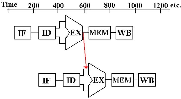
There is no stall. The value that will be written to $s0 is forwarded to the subtract
instruction just in time to be used. The value produced by the subtract instruction
is the correct value: $t0 + $t1 – $t3.

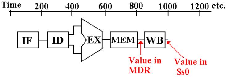
Load–Use Data Hazards

Suppose that we had the following sequence of instructions.

lw $s0, 100($gp) # Load a static variable

sub $t2, $s0, $t3 # $t2 = $s0 - $t3

If we examine the sequence of steps in executing the load word instruction, we
note that the new value of the register $s0 is not available until after the memory read.

If the code must be executed in exactly the sequence shown above, there is no avoiding a
pipeline stall. There will be one bubble if the value to be written to the register $s0 is
forwarded from the Memory Read stage of the Load Word instruction.

Forwarding for a Load–Use Data Hazard

This is a copy of Figure 4.30 from the textbook.

Possibly a clever compiler can insert a useful instruction after the “LW $s0”;
this would be one that does not reference the register just loaded.

Using a Clever Compiler

Often a compiler can reorder the obvious sequence to provide a sequence
that is less likely to stall.

Consider the code sequence: A = B + E;
C = B + F;

A straightforward compilation would yield something like the follow, which is
written in pseudo–MIPS assembly language.

LW $T1, B #$T1 GETS VALUE OF B

LW $T2, E #T2 GETS VALUS OF E

ADD $T3, $T1, $T2 #DATA HAZARD.ON $T2

SW $T3, A

LW $T4, F

ADD $T5, $T1, $T4 #ANOTHER DATA HAZARD

SW $T5, C

Using a Clever Compiler (Part 2)

Again, here is the code sequence: A = B + E;
C = B + F;

A good compiler can emit a non–obvious, but correct, code sequence,
such as the following. This allows the pipeline to move without stalls.

LW $T1, B # $T1 GETS A

LW $T2, E # $T2 GETS E

LW $T4, F # AVOID THE BUBBLE

ADD $T3, $T1, $T2 # $T1 AND $T2 ARE BOTH READY

SW $T3, A # NOW $T4 IS READY

ADD $T5, $T1, $T4

SW $T5, C

Note that the reordered instruction sequence has the correct semantics; the effect of
each instruction sequence is the same as that of the other.

Moving the Load F instruction up has two effects.

1. It provides “padding” to allow the value of E to be available when needed.

2. It places two instructions between the load of F and the time the value is used.

A More Detailed Analysis of the Sequence

The above “hand waving” argument is not satisfactory. Let’s do a detailed analysis of
the first instruction sequence, corresponding to A = B + E, with the “padding” added.

Time	Load B	Load E	Load F	Add B, E	Store A
1	Fetch
2	Decode	Fetch
3	Calculate Address	Decode	Fetch
4	Memory Access. B.	Calculate Address	Decode	Fetch
5	Update $T1	Memory Access. E.	Calculate Address	Decode	Fetch
6		Update $T2	Memory Access. F.	Add $T1 and forwarded E	Decode
7			Update $T4	Update $T3	Calculate Address
8					Write memory

Notice that the values of each of B and E are available to the ADD instruction just
before they are needed. One has been stored in a register and the other is forwarded.

Control Hazards: Do We Take the Branch?

The idea of pipelining is to have more than one instruction in execution at any given
time. When a given instruction has been decoded, we want the next instruction to
have been fetched and to have begun the decoding stage.

Suppose that the instruction that has just been decoded is a conditional branch?
What will be the next instruction to be executed?

There are two possible solutions to this problem.

1. Stall the pipeline until the branch condition is fully evaluated.
Then fetch the correct instruction.

2. Predict the result of the branch and fetch a next instruction.
If the prediction is wrong, the results of the incorrectly fetched instruction
must be discarded and the correct instruction fetched.

It is here that we see another advantage of the MIPS design. Each instruction changes
the state of the computer only late in its execution. With the exception of the branch
instruction itself, no instruction changes the state until the fourth step in execution.

This fact allows the CPU to start executing an incorrect instruction and then to fetch
and load the correct instruction with no lasting effect from the incorrect one.

Branch Prediction and Delayed Branching

The more accurately the branch result can be predicted, the more efficiently
the correct next instruction can be fetched and issued into the pipeline.

We shall discuss some standard static prediction and dynamic prediction
mechanisms in a future lecture.

Delayed branching attempts to reorder the instruction execution so that the CPU can
always have something correct to execute while the conditional branch instruction is
being executed and the next instruction address determined.

Consider the following instruction sequence.

ADD $4, $5, $6

BEQ $1, $2, 40 #Compare the two registers
#Branch if equal.

If the branch is not taken, the following sequence is exactly the same.

BEQ $1, $2, 40

ADD $4, $5, $6

The delayed branch strategy will reorder the instructions as in the second sequence, and
issue the ADD instruction to the pipeline while the BEQ is under execution. The ADD
instruction will complete execution independently of the result of the BEQ.