Sample
Design:
A Controller
for a Simple Traffic Light
Assumption:
Two Linked Pairs of Traffic Lights
If
one light is Green, the “cross light” must be Red.
Assumed
Cycling Rules
One Light Cross Light Comments
Green Red Traffic moving on one street
Yellow Red Traffic on cross street must wait
for
this light to turn red.
Red Red Both lights are red for about
one
second.
Red Green Cross traffic now moves.
This
is the basic sequence for a traffic light without turn signals or
features such as an
“advanced green”, etc.
Name the
States
|
State |
Light 1 |
Light 2 |
Alias |
|
0 |
Red |
Red |
RR |
|
1 |
Red |
Green |
RG |
|
2 |
Red |
Yellow |
RY |
|
3 |
Red |
Red |
RR |
|
4 |
Green |
Red |
GR |
|
5 |
Yellow |
Red |
YR |
Step 1a:
State Diagram for the System
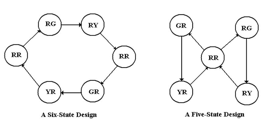
Notation:
L1L2, so RG Þ Light 1 is Red and Light 2 is Green
The six–state design is more
easily implemented.
Step 1b:
Define the State Table
|
Present State |
Next State |
||
|
Number |
Alias |
Number |
Alias |
|
0 |
RR |
1 |
RG |
|
1 |
RG |
2 |
RY |
|
2 |
RY |
3 |
RR |
|
3 |
RR |
4 |
GR |
|
4 |
GR |
5 |
YR |
|
5 |
YR |
0 |
RR |
At the moment, this is
just a modulo–6 counter with unusual output.
We
shall add some additional circuitry to allow for safety constraints.
The
choice of Red – Red as state 0 is arbitrary, but convenient.
Step 2: Count the States and
Determine the Flip–Flop Count
There
are six states, so we have N = 6.
Solve
2P–1 < N £ 2P for P, the number of flip–flops.
2P–1
< 6 £ 2P gives P =
3, because 22 < 6 £ 23.
We
denote the states by Q2Q1Q0, because the
symbol “Y” is taken to
indicate the color Yellow.
Step 3:
Assign a 3–bit Binary Number
to Each State
This
is a modified counter, so the assignments are quite obvious.
|
State |
Q2 |
Q1 |
Q0 |
|
0 |
0 |
0 |
0 |
|
1 |
0 |
0 |
1 |
|
2 |
0 |
1 |
0 |
|
3 |
0 |
1 |
1 |
|
4 |
1 |
0 |
0 |
|
5 |
1 |
0 |
1 |
We have two possible additional
states: 6 and 7.
Normally, these are ignored,
but we consider them due to
safety constraints.
Redefine the
State Diagram to Add Safety
States
6 and 7 should never be entered. Each is
“RR” for safety.
Step 4a:
Derive the Output Equations.
|
|
Alias |
Q2Q1Q0 |
R1 |
G1 |
Y1 |
R2 |
G2 |
Y2 |
|
0 |
RR |
0 0 0 |
1 |
0 |
0 |
1 |
0 |
0 |
|
1 |
RG |
0 0 1 |
1 |
0 |
0 |
0 |
1 |
0 |
|
2 |
RY |
0 1 0 |
1 |
0 |
0 |
0 |
0 |
1 |
|
3 |
RR |
0 1 1 |
1 |
0 |
0 |
1 |
0 |
0 |
|
4 |
GR |
1 0 0 |
0 |
1 |
0 |
1 |
0 |
0 |
|
5 |
YR |
1 0 1 |
0 |
0 |
1 |
1 |
0 |
0 |
|
6 |
RR |
1 1 0 |
1 |
0 |
0 |
1 |
0 |
0 |
|
7 |
RR |
1 1 1 |
1 |
0 |
0 |
1 |
0 |
0 |
Here are the output
equations
G1 = Q2·Q1’·Q0’ G2
= Q2’·Q1’·Q0
Y1 = Q2·Q1’·Q0 Y2
= Q2’·Q1·Q0’
R1 = (G1 + Y1)’ R2 = (G2 + Y2)’
Step 4a:
Derive the Output Equations.
(page 2)
Here
are the equations again.
G1
= Q2·Q1’·Q0’ G2 = Q2’·Q1’·Q0
Y1
= Q2·Q1’·Q0 Y2 = Q2’·Q1·Q0’
R1
= (G1 + Y1)’ R2 = (G2 + Y2)’
We
derive the Green and Yellow signals, which are easier.
We stipulate that if a light is not Green or Yellow, it must be Red.
Now
add a safety constraint: If a light is Green or Yellow, the
cross light must be Red.
R1 = (G1 + Y1)’ + G2 + Y2, and
R2 = (G2 + Y2)’ + G1 + Y1
These equations may lead to a
light showing two colors.
This is obviously an error
situation.
Step 4b:
Derive the State Transition Table.
|
Present
State |
Next State |
|
|
|
Q2Q1Q0 |
Q2Q1Q0 |
|
0 |
0 0 0 |
0 0 1 |
|
1 |
0 0 1 |
0 1 0 |
|
2 |
0 1 0 |
0 1 1 |
|
3 |
0 1 1 |
1 0 0 |
|
4 |
1 0 0 |
1 0 1 |
|
5 |
1 0 1 |
0 0 0 |
|
6 |
1 1 0 |
0 0 0 |
|
7 |
1 1 1 |
0 0 0 |
Step 5:
Separate the Table into Three Tables
|
Q2 |
|
Q1 |
|
Q0 |
|||
|
PS |
NS |
|
PS |
NS |
|
PS |
NS |
|
Q2Q1Q0 |
Q2 |
|
Q2Q1Q0 |
Q1 |
|
Q2Q1Q0 |
Q0 |
|
0 0 0 |
0 |
|
0 0 0 |
0 |
|
0 0 0 |
1 |
|
0 0 1 |
0 |
|
0 0 1 |
1 |
|
0 0 1 |
0 |
|
0 1 0 |
0 |
|
0 1 0 |
1 |
|
0 1 0 |
1 |
|
0 1 1 |
1 |
|
0 1 1 |
0 |
|
0 1 1 |
0 |
|
1 0 0 |
1 |
|
1 0 0 |
0 |
|
1 0 0 |
1 |
|
1 0 1 |
0 |
|
1 0 1 |
0 |
|
1 0 1 |
0 |
|
1 1 0 |
0 |
|
1 1 0 |
0 |
|
1 1 0 |
0 |
|
1 1 1 |
0 |
|
1 1 1 |
0 |
|
1 1 1 |
0 |
Color
added to emphasize the transitions of interest.
Step 6:
Select the Flip–Flops to Use
Use
JK flip–flops. What a surprise!
The
excitation table for a JK flip-flop is given again.
|
Q(T) |
Q(T + 1) |
|
J |
K |
|
0 |
0 |
|
0 |
d |
|
0 |
1 |
|
1 |
d |
|
1 |
0 |
|
d |
1 |
|
1 |
1 |
|
d |
0 |
Step 7: Derive
the Input Tables
|
Flip-Flop 2 |
|
Flip-Flop 1 |
|
Flip-Flop 0 |
|||||||||
|
PS |
NS |
Input |
|
PS |
NS |
Input |
|
PS |
NS |
Input |
|||
|
Q2Q1Q0 |
Q2 |
J2 |
K2 |
|
Q2Q1Q0 |
Q1 |
J1 |
K1 |
|
Q2Q1Q0 |
Q0 |
J0 |
K0 |
|
0 0 0 |
0 |
0 |
d |
|
0 0 0 |
0 |
0 |
d |
|
0 0 0 |
1 |
1 |
d |
|
0 0 1 |
0 |
0 |
d |
|
0 0 1 |
1 |
1 |
d |
|
0 0 1 |
0 |
d |
1 |
|
0 1 0 |
0 |
0 |
d |
|
0 1 0 |
1 |
d |
0 |
|
0 1 0 |
1 |
1 |
d |
|
0 1 1 |
1 |
1 |
d |
|
0 1 1 |
0 |
d |
1 |
|
0 1 1 |
0 |
d |
1 |
|
1 0 0 |
1 |
d |
0 |
|
1 0 0 |
0 |
0 |
d |
|
1 0 0 |
1 |
1 |
d |
|
1 0 1 |
0 |
d |
1 |
|
1 0 1 |
0 |
0 |
d |
|
1 0 1 |
0 |
d |
1 |
|
1 1 0 |
0 |
d |
1 |
|
1 1 0 |
0 |
d |
1 |
|
1 1 0 |
0 |
0 |
d |
|
1 1 1 |
0 |
d |
1 |
|
1 1 1 |
0 |
d |
1 |
|
1 1 1 |
0 |
d |
1 |
Step 8: Derive
the Input Equations
Here they are
J2
= Q1 · Q0 J1
= Q2’ · Q0 J0
= Q2’ + Q1’
K2 = Q1
+ Q0 K1 = Q2
+ Q0 K0
= 1
There
is no need to summarize the equations.
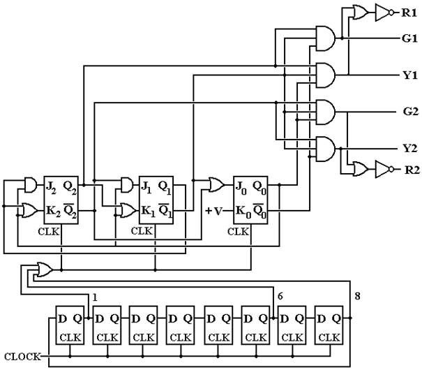
Step 10:
Draw the Circuit