Chapter 18 – The Cray Line of Supercomputers

We now turn to a discussion of the most significant line of supercomputers from the 20^th century. Admittedly, we could also say the last third of the 20^th century as there were no supercomputers, in any sense of the word, until about 1964 when the CDC–6600 was introduced. The year 1964 was also the year that the IBM System/360 was announced. This is considered a mainframe computer and not a supercomputer.

The difference between a mainframe and a supercomputer is entirely a matter of definition, though one that does make sense. A supercomputer is a large powerful computer that is designed to bring computational power to solution of a single large problem. It solves one problem at a time. A mainframe should be considered as a transaction processor, though this is not strictly necessary. Each transaction is quite simple: update a bank balance, print a payroll check, post an airline reservation, etc. What makes the mainframe unique is its ability to handle massive numbers of transactions per unit time, and to do so with very high reliability. Mainframes and supercomputers address different classes of problems.

Within the confines of this chapter, we shall use the terms “supercomputer” and “vector processor” as synonyms, as they were used for about 25 years. The first vector processor was the Cray–1, designed by Seymour Cray, installed in Los Alamos National Lab in 1976. The term “vector processor” is distinguished from “scalar processor” in the literature.

The terms “scalar” and “vector” are adopted from the field of mathematics, and retain their definitions. A scalar is a number of a number of varieties, typically integer or real. It is true that complex numbers are also scalars in the mathematical sense, but they are treated differently in computer science. A vector is just a collection of scalar quantities; e.g., the (X, Y, Z) coordinates of a point. In this field, we ignore the difference between the coordinates of a point and the vector from the origin of coordinates to that point.

The difference between scalar and vector designs can be seen in the following FORTRAN fragment. Each adds two arrays to produce a third array.

DO 200, I = 1, 1000
DO 200, J = 1, 1000
C(I, J) = A(I, J) + B(I, J)
200 CONTINUE

Each of A(I, J), B(I, J), and C(I, J) is a scalar element of its respective array. In a scalar processor, the key instruction is the statement C(I, J) = A(I, J) + B(I, J). This will be put in a loop and executed a million times. In a vector processor, there is more of the flavor of a vector addition: C = A + B. Here there would be no loop structure, and the key instruction would be fetched from memory only once, rather than one million times, as in the scalar processor. As we shall see later, the vector processor uses a particularly safe form of pipelining, one that has few data hazards.

The Cray series of computers, which are the subject of this chapter, were equipped with both scalar and vector execution units. When operated only in scalar mode, the computer would become a standard processor, though a fairly powerful one.

The Cray–1, delivered in 1976, was the first of the Cray line of supercomputers, and the first true vector processor. It was an immediate hit among scientists who needed considerable computational power, mostly because the vector facilities seemed a perfect match to the array–heavy computation that was the life work of these scientists. Below is a figure of the Cray–1 at the Deutsches Museum in Munich Germany.

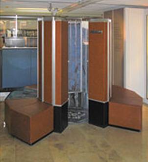
Figure: The Cray–1 at the Deutsches Museum in Munich Germany

Note the design. The low parts contained the power supplies for the computer proper, which was housed in the taller parts. In 1976, the magazine Computerworld called the Cray–1
“the world’s most expensive love seat”.

History of Seymour Cray and His Companies

In order to understand the Cray line of computers, we must look at the personal history of Seymour Cray, the “father of the supercomputer”. Cray began work at Control Data Corporation soon after its founding in 1960 and remained there until 1972. He designed several computers, including the CDC 1604, CDC 6600, and CDC 7600. The CDC 1604 was intended just to be a good computer; all computers beginning with the CDC 6600 were designed for speed. The CDC 6600 is often called the first RISC (Reduced Instruction Set Computer), due to the simplicity of its instruction set. The reason for its simplicity was the desire for speed. Cray also put a lot of effort into matching the memory and I/O speed with the CPU speed. As he later noted, “Anyone can build a fast CPU. The trick is to build a fast system.” Full disclosure: Your author has programmed on the CDC 6600, CDC 7600, and Cray–1; he found each to be excellent machines with very clean architectures.

The CDC 6600 lead to the more successful CDC 7600. The CDC 8600 was to be a follow–on to the CDC 7600. While an excellent design, it proved too complex to manufacture successfully, and was abandoned. Cray left Control Data Corporation in 1972 to found Cray Research, based in Chippewa Falls, Wisconsin. The main reason for his departure was the fact that CDC could not bankroll his project leading to development of the Cray–1. The parting was cordial; CDC did invest some money in Cray’s new company.

In 1989, Cray left Cray Research in order to found Cray Computers, Inc. His reason for leaving was that he wanted to spend more time on research, rather than just churning out the very profitable computers that his previous company was manufacturing. This lead to an interesting name game:

Cray Research, Inc. producing a large number of commercial computers

Cray Computer, Inc. mostly invested in research on future machines.

The Cray–3, a 16–processor system, was announced in 1993 but never delivered. The
Cray–4, a smaller version of the Cray–3 with a 1 GHz clock was ended when the Cray Computer Corporation went bankrupt in 1995. Seymour Cray died on October 5, 1996.

In 1993, Cray Research moved away from pure vector processors, producing its first massively parallel processing (MPP) system, the Cray T3D™. We shall discuss this decision a bit later, in another chapter of this book, when we discuss the rise of MPPs. Cray Research merged with SGI (Silicon Graphics, Inc.) in February 1996. It was spun off as a separate business unit in August 1999. In March 2000, Cray Research was merged with Terra Computer Company to form Cray, Inc. The company still exists and has a very nice web site (www.cray.com).

Here is a schematic of the Cray–1. At the base, it is more than 8 feet in diameter.

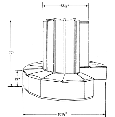
We may think this a large computer, but for its time the Cray–1 was surprisingly small. Your author recalls the first time he actually saw a Cray–1. The first thought was “Is this all there is?” Admittedly, there were a number of other units associated with this, including disk farms, tape drives, and a variety of other I/O devices. As your author recalls, there was a dedicated Front End Processor, possibly a CDC–7600, to manage the tapes and disks. The division of work load into computational and I/O has a long history, for the reason it works.

Processor Specifications of the Cray–1

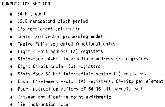
Source: Cray–1 Computer System Hardware Reference Manual
Publication 2240004, Revision C, November, 1977 [R106].

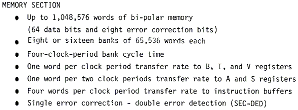
Note that the memory size, without error correction, would be 8MB. Each word has 64 data bits (8 bytes) as well as 8 bits for error correction. Other material indicates that the memory was low–order interleaved.

Here is a considerable surprise. We are discussing what was agreed to be the most powerful computer of the late 1970’s. Yet it had only eight megabytes of memory. The reader is invited to revisit this textbook’s chapter on memory and note the price of memory in 1976.

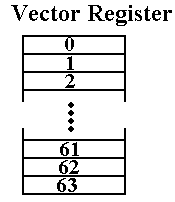
The Cray–1 Vector Registers

It is important to understand the structure and function of the vector registers, as it is this set of structures that made the computer a vector processor. Each of the vector registers is a vector of registers, best viewed as a collection of sixty–four registers each holding 64 bits. A vector register held 4,096 bits. Vector registers are loaded from primary memory and store results back to primary memory. One common use would be to load a vector register from sixty–four consecutive memory words. Nonconsecutive words could be handled if they appeared in a regular pattern, such as every other word or every fourth word, etc.

One might consider each register as an array, but that does not reflect its use. One of
the key design features of the Cray is the placement of a large number of registers
between the memory and the CPU units. These function much as cache memory.

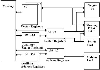
Note that the scalar and address registers also have auxiliary registers.

In some sense, we can say that the T registers function as a cache for the S registers, and the B registers function as a cache for the A registers. Without the register storage provided by the B, T, and V registers, the CRAY–1’s [memory] bandwidth of only 80 million words per second would be a serious impediment to performance. Each word is 8 bytes; 80 million words per second is 640 million bytes per second, or one byte every 1.6 nanoseconds.

Advantages of Vector Processors

Note that many of the advantages of a vector processor depend on the structure of the problem for which the program has been written.

“Advantages of vector computers over traditional SISD processors include the following:

1. Each result is independent of previous results, which enables deep pipelines and high clock rates without generating any data hazards.

2. A single vector instruction performs a great deal of work, which means fewer instruction fetches in general, and fewer branch instructions and so fewer mispredicted branches.

3. Vector instructions access memory a block at a time, which allows memory latency to be amortized over, say, 64 elements.

4. Vector instructions access memory with known patterns, which allows multiple memory banks to simultaneously supply operands.

These last two advantages mean that vector processors do not need to rely on high hit rates of data caches to have high performance. They tend to rely on low-latency main memory, often made from SRAM, and have as many as 1024 memory banks to get high memory bandwidth.” [R80]

Amount of Work

Note that the single vector instruction can correspond to the execution of 64 scalar instructions in a normal SISD architecture. This makes very good use of the bandwidth to the Instruction Cache that fronts the memory. One instruction is fetched and does the work of sixty four, with 63 fewer instruction fetches. Remember that the goal is to make the best use of primary memory, which is inherently much slower than the CPU execution units.

Locality of Memory Access

All vector instructions accessing memory have a predictable access pattern. This pattern provides a good match for an interleaved primary memory, of the type we discussed in a previous lecture on matching the cache and main memory. Consider a vector with 64 entries, each a 64–bit double word. The vector has size of 512 bytes. Given a heavily interleaved memory (1024–way is not uncommon) the cost to access the first byte to be transferred is amortized over the entire vector. If it takes 80 nanoseconds to retrieve the first byte and 4 nanoseconds each to retrieve the remaining 511, the average access time is
(80 + 4·511)/512 = 2124/512 = 4.15 ns.

Control Hazards

Most of the control hazards in a scalar unit have to do with conditional branches, such as taken at the end of a loop. Many of these loops are now represented as a single vector instruction, which obviously has no branch hazard.

The only branch hazards in a vector pipeline occur due to conditional branches, such as the IF … THEN … ELSE tests.

Evolution of the Cray–1

In this course, the main significance of the CDC 6600 and CDC 7600 computers lies in their influence on the design of the Cray–1 and other computers in the series. Remember that Seymour Cray was the principle designer of all three computers.
Here is a comparison of the CDC 7600 and the Cray–1.

Item CDC 7600 Cray–1

Circuit Elements Discrete Components Integrated Circuitry

Memory Magnetic Core Semiconductor (50 nanoseconds)

Scalar (word) size 60 bits 64 bits (plus 8 ECC bits)

Vector Registers None Eight, each holding 64 scalars.

Scalar Registers Eight: X0 – X7 Eight: S0 – S7

Scalar Buffer Registers None Sixty–four T0 – T77
Octal numbering was used.

Address Registers Eight: A0 – A7 Eight: A0 – A7

Address Buffer Registers None Sixty–four: B0 – B77

Two main changes: 1. Addition of the eight vector registers.
2. Addition of fast buffer registers for the A and S registers.

Chaining in the Cray–1

Here is how the technique is described in the 1978 article [R107].

“Through a technique called ‘chaining’, the CRAY–1 vector functional units, in combination with scalar and vector registers, generate interim results and use them again immediately without additional memory references, which slow down the computational process in other contemporary computer systems.”

This is exactly the technique, called “forwarding”, used to handle data hazards in a pipelined control unit. Essentially a result to be written to a register is made available to computational units in the CPU before it is stored back into the register file.

Consider the following example using the vector multiply and vector addition operators.

MULTV V1, V2, V3 // V1[K] = V2[K] · V3[K]

ADDV V4, V1, V5 // V4[K] = V1[K] + V5[K]

Without chaining (forwarding), the vector multiplication operation would have to finish before the vector addition could begin. Chaining allows a vector operation to start as soon as the individual elements of its vector source become available. The only restriction is that operations being chained belong to distinct functional units, as each functional unit can do only one thing at a time.

Vector Startup Times

Vector processing involves two basic steps: startup of the vector unit and pipelined operation. As in other pipelined designs, the maximum rate at which the vector unit executes instructions is called the “Initiation Rate”, the rate at which new vector operations are initiated when the vector unit is running at “full speed”.

The initiation rate is often expressed as a time, so that a vector unit that operated at
100 million operations per second would have an initiation rate of 10 nanoseconds. The time to process a vector depends on the length of the vector. For a vector with length N (containing N elements) we have
T(N) = Start–Up_Time + N·Initiation_Rate

The time per result is then T = (Start–Up Time) / N + Initiation_Rate. For short vectors (small values of N), this time may exceed the initiation rate of the scalar execution unit. An important measure of the balance of the design is the vector size at which the vector unit can process faster than the scalar unit. For a Cray–1, this crossover size was between 2 and 4;
2 £ N £ 4. For N > 4, the vector unit was always faster.

Here are some comparative data for mathematical operations (Log, cosine, square root, and exponential), showing the per–result times as a function of vector length. Note the low crossover point, for vectors larger than N = 5, the vector unit is much faster.

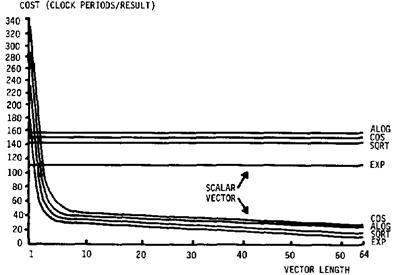
The time cost is given in clock ticks, not nanoseconds. See Russell, 1978 [R107].

The Cooling Issue

The CRAY–1 computer weighed 5.25 tons (10,500 pounds or 4773 kilograms). It consumed 130 kilowatts of power. All that power emerged as heat. The problem was keeping the computer cool enough to operate. The goal was not to keep the semiconductor circuitry from melting, but to keep it from rising to the temperature at which thermal noise made it inoperable. Thermal noise refers to the fact that all semiconductors generate electric signals as a result of their temperature. The maximum voltage of the signals due to thermal noise increase as the temperature increases; for reasonable temperatures they are so much smaller than the voltages intentionally generated that they can be ignored.

The CRAY–1 and its derivative computers (CRAY X–MP and CRAY Y–MP, etc.) employed a cold plate approach to cooling. All circuit elements were mounted on a ground plane (used to assert zero volts) that was a copper sheet also used to cool the circuit. The copper sheet was attached to an aluminum cold bar, maintained at 25 Celsius by a Freon refrigerant flowing through stainless steel tubes.

It is worth note that it took a year and a half before the first good cold bar was built. A major problem was the discovery that Aluminum is porous. The difficulty was not due to loss of Freon, but due to the oil that contaminated the Freon; it could damage the circuits.

The Cray X–MP and Cray Y–MP

The fundamental tension at Cray Research, Inc. was between Seymour Cray’s desire to develop new and more powerful computers and the need to keep the cash flow going. Seymour Cray realized the need for a cash flow at the start. As a result, he decided not to pursue his ideas based on the CDC 8600 design and chose to develop a less aggressive machine. The result was the Cray–1, which was still a remarkable machine.

With its cash flow insured, the company then organized its efforts into two lines of work.

1. Research and development on the CDC 8600 follow–on, to be called the Cray–2.

2. Production of a line of computers that were derivatives of the Cray–1 with
improved technologies. These were called the X–MP, Y–MP, etc.

The X–MP was introduced in 1982. It was a dual–processor computer with a 9.5 nanosecond (105 MHz) clock and 16 to 128 megawords of static RAM main memory.
A four–processor model was introduced in 1984 with a 8.5 nanosecond clock.

The Y–MP was introduced in 1988, with up to eight processors that used VLSI chips.
It had a 32–bit address space, with up to 64 megawords of static RAM main memory.

The Y–MP M90, introduced in 1992, was a large–memory variant of the Y–MP that replaced the static RAM memory with up to 4 gigawords of DRAM.

The Cray–2

While his assistant, Steve Chen, oversaw the production of the commercially successful
X–MP and Y–MP series, Seymour Cray pursued his development of the Cray–2, a design based on the CDC 8600, which Cray had started while at the Control Data Corporation. The original intent was to build the VLSI chips from gallium arsenide (GaAs), which would allow must faster circuitry. The technology for manufacturing GaAs chips was not then mature enough to be useful as circuit elements in a large computer.

The Cray–2 was a four–processor computer that had 64 to 512 megawords of 128–way interleaved DRAM memory. The computer was built very small in order to be very fast, as a result the circuit boards were built as very compact stacked cards. Note the hand holding the stacked circuitry in the figure below.

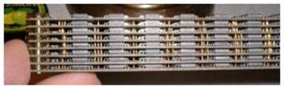
Due to the card density, it was not possible to use air cooling. The entire system was immersed in a tank of Fluorinert™, an inert liquid intended to be a blood substitute. When introduced in 1985, the Cray–2 was not significantly faster than the Y–MP. It sold only thirty copies, all to customers needing its large main memory capacity.

Whatever Happened to Gallium Arsenide?

In his 1981 paper on the CRAY–1, J. S. Kolodzev listed the advantages of Gallium Arsenide as a semiconductor material and hinted that future Cray computers would use circuits fabricated from the material. Whatever happened?

It is true that the one and only CRAY–3 was build with GaAs circuits. This was shortly before the Cray Computer Company went bankrupt.

The advantages of Gallium Arsenide are seen in the following table of switching times.

Material	Switching Speed	Relative to Silicon
Silicon	400 picoseconds	1
Gallium Arsenide	80 picoseconds	5 times faster
Josephson Junction	15 picoseconds	27 times faster

The clear winner is the Josephson junction. The difficulty is that it only operates at superconducting temperatures, which at the time were 4 Kelvins (– 452 F), the temperature of liquid Helium. The discovery of high–temperature superconducting in the late 1980’s may push this up to 77 Kelvins (– 321 F), the temperature of liquid Nitrogen.

Operation of any circuitry at 4 Kelvins requires use of liquid Helium, which is expensive. Operation at 77 Kelvins requires use of liquid Nitrogen, which is plentiful and cheap. Nevertheless, most computer operators do not want to bother with it. This option is out.

Why not Gallium Arsenide?

Why not Gallium Arsenide? It was hard to fabricate and, unlike Silicon, did not form a stable oxide that could be used as an insulator. This made Silicon the preferred choice for the new high–speed circuit technology, called CMOS, which was increasingly used in the late 1980’s and 1990’s. The economy of scale available to the Silicon industry also played a large role in inhibiting the adoption of Gallium Arsenide. This is another example of the mass market products that are good enough for the job freezing out the low market, high technology, products that theoretically are better.

The Cray–3 and the End of an Era

After the Cray–2, Seymour Cray began another very aggressive design: the Cray–3. This was to be a very small computer that fit into a cube one foot on a side. Such a design would require retention of the Fluorinert cooling system. It would also be difficult to manufacture as it would require robotic assembly and precision welding. It would also have been very difficult to test, as there was no direct access to the internal parts of the machine.

The Cray–3 had a 2 nanosecond cycle time (500 MHz). A single processor machine would have a performance of 948 megaflops; the 16–processor model would have operated at 15.2 gigaflops. The 16–unit model was never built. The Cray–3 was delivered in 1993. In 1994, Cray Research, Inc. released the T90 with a 2.2 nanosecond clock time and eight times the performance of the Cray–3.

In the end, the development of traditional supercomputers ran into several problems.

1. The end of the cold war reduced the pressing need for massive computing facilities.

2. The rise of microprocessor technology allowing much faster and cheaper processors.

3. The rise of VLSI technology, making multiple processor systems more feasible.

Supercomputers vs. Multiprocessor Clusters

“If you were plowing a field, which would you rather use: Two
strong oxen or 1024 chickens?” Seymour Cray

Although Seymour Cray said it more colorfully, there were many objections to the transition from the traditional vector supercomputer (with a few processors) to the massively parallel computing that replaced it. Here we quote from an overview article written in 1984 [R108]. It assessed the commercial viability of traditional vector processors and multiprocessor systems. The key issue in assessing the commercial viability of a multiple–processor system is the speedup factor; how much faster is a processor with N processors. Here are two opinions from the 1984 IEEE tutorial on supercomputers [R108].

“The speedup factor of using an n–processor system over a uniprocessor system has been theoretically estimated to be within the range (log₂n, n/log₂n). For example, the speedup range is less than 6.9 for n = 16. Most of today’s commercial multiprocessors have only 2 to 4 processors in a system.”

“By the late 1980s, we may expect systems of 8–16 processors. Unless the technology changes drastically, we will not anticipate massive multiprocessor systems until the 90s.”

As we shall see soon, technology has changed drastically.