Stacks and Recursion

NUMOUT: The Newer Version

The newer version of NUMOUT will be written in the style required for recursive subroutines, although it will not be recursive.
This style requires explicit management of the return address. This requires the definition of a label for the instruction following
the call to NUMOUT. For no particular reason, this statement is called NUMRET.

MVC PRINT,BLANKS CLEAR THE OUTPUT BUFFER

LA 8,NUMRET STATEMENT AFTER NUMOUT

STKPUSH R8,R PLACE ADDRESS ONTO STACK

B NUMOUT BRANCH DIRECTLY TO NUMOUT

NUMRET MVC DATAPR,THENUM AND COPY TO THE PRINT AREA

Here is the new code for NUMOUT.

NUMOUT CVD R4,PACKOUT CONVERT TO PACKED

UNPK THENUM,PACKOUT PRODUCE FORMATTED NUMBER

MVZ THENUM+7(1),=X’F0’ CONVERT SIGN HALF-BYTE

STKPOP R8,R POP THE RETURN ADDRESS

BR 8 RETURN ADDRESS IN R8

Factorial: A Recursive Function

One of the standard examples of recursion is the factorial function. We shall give its standard recursive definition and
then show some typical code.

Definition: If N £ 1, then N! = 1
Otherwise N! = N·(N – 1)!

Here is a typical programming language definition of the factorial function.

Integer Function FACT(N : Integer)

If N £ 1 Then Return 1

Else Return N*FACT(N – 1)

Such a function is easily implemented in a compiled high–level language (such as C++
or Java) that provides a RTS (Run Time System) with native support of a stack. As we shall see, a low–level language,
such as IBM 370 assembler, must be provided with explicit stack handling routines if recursion is to be implemented.

Tail Recursion and Clever Compilers

Compilers for high–level languages can generally process a construct that is “tail recursive”, in which the recursive call
is the last executable statement. Consider the above code for the factorial function.

Integer Function FACT(N : Integer)

If N £ 1 Then Return 1

Else Return N*FACT(N – 1)

Note that the recursive call is the last statement executed when N > 1.

A good compiler will turn the code into the following, which is equivalent.

Integer Function FACT(N : Integer)

Integer F = 1 ; Declare a variable and initialize it

For (K = 2, K++, K <= N) Do F = F*K ;

Return F ;

This iterative code consumes fewer RTS resources and executes much faster.
NOTE: For fullword (32–bit integer) arithmetic, the biggest we can calculate is 12!

A Pseudo–Assembler Implementation with Problems

We want an implementation of the factorial function. It takes one argument and returns one value. We shall attempt
an implementation as FACTOR, with each of the argument and
result being passed in register R4 (my favorite). It might be called as follows.

L 4,THEARG

BAL 8,FACTOR

N1 ST 4,THERESULT

Pseudocode for the function might appear as follows.

If (R4 £ 1) Then

L R4, = F’1’ SET R4 EQUAL TO 1

A1 BR 8 RETURN TO CALLING ROUTINE

Else

LR 7,4 COPY R4 INTO R5

S 4,=F’1’

BAL 8,FACTOR

N2 MR 6,4 MULTIPLY

A2 BR 8

This code works only for N £ 1.

Confusion with the Return Addresses

Suppose that FACTOR is called with N = 1. The following code executes.

L 4,=F’1’

BAL 8,FACTOR The first call to FACTOR

N1 ST 4,THERESULT

If (R4 £ 1) then the function code is invoked. This is all that happens.

L R4, = F’1’ SET R4 EQUAL TO 1

A1 BR 8 RETURN TO CALLING ROUTINE

But note at this point, register 8 contains the address N1. Return is normal.

Suppose now that FACTOR is called with N = 2.

L 4,=F’2’

BAL 8,FACTOR PLACE A(N1) INTO R8

N1 ST 4,THERESULT

This code is executed.

LR 7,4 COPY R4 INTO R5

S 4,=F’1’

BAL 8,FACTOR PLACE A(N2) INTO R8

N2 MR 6,4 MULTIPLY

A2 BR 8

The above call causes the following code to execute, as N = 1 now.

L R4, = F’1’ SET R4 EQUAL TO 1

A1 BR 8 RETURN TO CALLING ROUTINE

Here is the trouble. For N = 1, the return is OK.

Back at the invocation for N = 2. Compute 2·1 = 2.

Try to return to N1. But R8 contains the address N2.

The code is “trapped within FACTOR”. It can never return to the main program.

Outline of the Solution

Given the limitations of the IBM 370 original assembly language, the only way to implement recursion is to
manage the return addresses ourselves. This must be done by explicit use of the stack. Given that we are
handling the return addresses directly, we dispense with the BAL instruction and use the unconditional branch instruction, B.

Here is code that shows the use of the unconditional branch instruction.
At this point, register R4 contains the argument.

LA R8,A94PUTIT ADDRESS OF STATEMENT AFTER CALL

STKPUSH R8,R PUSH THE ADDRESS ONTO THE STACK

STKPUSH R4,R PUSH THE ARGUMENT ONTO THE STACK

B DOFACT CALL THE SUBROUTINE

A94PUTIT BAL 8,NUMOUT FINALLY, RETURN HERE.

Note that the address of the return instruction is placed on the stack. Note also that the return target uses the
traditional subroutine call mechanism. In this example, the goal is to focus on recursion in the use of the DOFACT
subprogram. For NUMOUT, we shall use the standard subroutine linkage based on the BAL instruction.

Proof of Principle: Code Fragment 1

Here is the complete code for the first proof of principle. The calling code is as follows.
The function is now called DOFACT.

LA R8,A94PUTIT ADDRESS OF STATEMENT AFTER CALL

STKPUSH R8,R PUSH THE ADDRESS ONTO THE STACK

STKPUSH R4,R PUSH THE ARGUMENT ONTO THE STACK

B DOFACT CALL THE SUBROUTINE

A94PUTIT BAL 8,NUMOUT FINALLY, RETURN HERE.

The first test case was designed with a stub for DOFACT. This design was to prove the return mechanism.
The code for this “do nothing” version of DOFACT is as follows.

DOFACT STKPOP R4,R POP RESULT BACK INTO R4

STKPOP R8,R POP RETURN ADDRESS INTO R8

BR 8 BRANCH TO THE POPPED ADDRESS

Remember: 1. STKPOP R4,R is a macro invocation.

2. The macros have to be written with a symbolic parameter as
the label of the first statement.

The Stack for Both Argument and Return Address

We now examine a slightly non–standard approach to using the stack to store both arguments to the function
and the return address. In general, the stack can be used to store any number of arguments to a function or
subroutine. We need only one argument, so that is all that we shall stack.

Remember that a stack is a Last In / First Out data structure.

It could also be called a First In / Last Out data structure; this is seldom done.

Recall the basic structure of the function DOFACT. Here is the skeleton.

DOFACT

Use the argument from the stack

STKPOP R8,R POP RETURN ADDRESS INTO R8

BR 8 BRANCH TO THE POPPED ADDRESS

Since the return address is the last thing popped from the stack when the routine returns,
it must be the first thing pushed onto the stack when the routine is being called.

Basic Structure of the Function

On entry, the stack has both the argument and return address. On exit, it must
have neither. The return address is popped last, so it is pushed first.

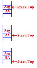
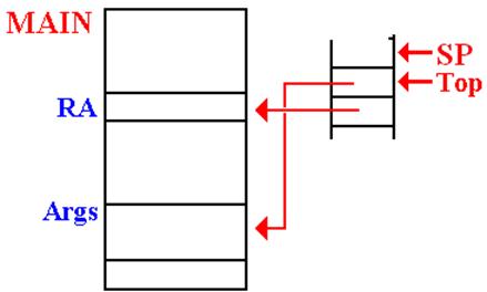
On entry to the routine, this is the status of the stack. By “Stack Top”, I indicate the
location of the last item pushed.

At some point, the argument must be popped from the stack, so that the Return Address
is available to be popped.

STKPOP 8 Get the return address
BR 8 Go there

Note that the contents of the stack are not removed. This is in line with standard stack
protocol, though it might have some security implications.

When Do We Pop the Argument?

The position of the STKPOP depends on the use of the argument sent to the function. There are two considerations,
both of which are quite valid. Assume that register R7 contains the argument. We shall get it there on the next slide.
Consider the fragment of code corresponding to N·FACT(N – 1).

FDOIT S R7,=F'1' SUBTRACT 1 FOR NEW ARGUMENT

LA 8,FRET GET THE ADDRESS OF RETURN

STKPUSH R8,R STORE NEW RETURN ADDRESS

STKPUSH R7,R NOW, PUSH NEW ARG ONTO STACK

B DOFACT MAKE RECURSIVE CALL

FRET L R2,=F'0'

At this point, the return register (say R4) will contain FACT(N – 1).

At this point, the value of N should be popped from the stack and multiplied by the result
to get the result N·FACT(N – 1), which will be placed into R4 as the return value. But recall that the basic
structure of the factorial function calls for something like:

STKPOP R7,R

If the value in R7 is not greater than 1, execute this code.

L R4,=F’1’ SET THE RETURN VALUE TO 1

STKPOP R8,R POP THE RETURN ADDRESS

BR 8 RETURN TO THE CALLING ROUTINE.

If the value in R7 is larger than 1, then execute this code.

FDOIT S R7,=F'1' SUBTRACT 1 FOR NEW ARGUMENT

LA 8,FRET GET THE ADDRESS OF RETURN

STKPUSH R8,R STORE NEW RETURN ADDRESS

STKPUSH R7,R NOW, PUSH NEW ARG ONTO STACK

B DOFACT MAKE RECURSIVE CALL

FRET L R2,=F'0'

But, there is only one copy of the argument value. How can we pop it twice.

Answer: We push it back onto the stack.

Examining the Value at the Top of the Stack

Here is the startup code for the function DOFACT.

DOFACT L R2,=F'0'

STKPOP R7,R GET THE ARGUMENT AND EXAMINE

STKPUSH R7,R BUT PUT IT BACK ONTO THE STACK

C R7,=F'1' IS THE ARGUMENT BIGGER THAN 1

BH FDOIT YES, WE HAVE A COMPUTATION

This code fragment shows the strategy for examining the top of the stack without removing the value:
just pop it and push it back onto the stack. There is another common way of examining the top of the s
tack. Many stack implementations use a function STKTOP, which returns the value at the stack top
without removing it. We shall not use this option.

This is another valid option. That code could be written as follows.

DOFACT L R2,=F'0' SET R2 TO ZERO

STKTOP R7,R GET THE ARGUMENT VALUE

C R7,=F'1' IS THE ARGUMENT BIGGER THAN 1

BH FDOIT YES, WE HAVE A COMPUTATION

The Factorial Function DOFACT
Here is the code for the recursive version of the function DOFACT.

DOFACT STKPOP R7,R GET THE ARGUMENT AND EXAMINE

STKPUSH R7,R BUT PUT IT BACK ONTO THE STACK

C R7,=F'1' IS THE ARGUMENT BIGGER THAN 1

BH FDOIT YES, WE HAVE A COMPUTATION

L R4,=F'1' NO, JUST RETURN THE VALUE 1

STKPOP R7,R ARG IS NOT USED, SO POP IT

B FDONE AND RETURN

FDOIT S R7,=F'1' SUBTRACT 1 FOR NEW ARGUMENT

LA 8,FRET GET THE ADDRESS OF RETURN

STKPUSH R8,R STORE NEW RETURN ADDRESS

STKPUSH R7,R NOW, PUSH NEW ARG ONTO STACK

B DOFACT MAKE RECURSIVE CALL

FRET STKPOP R7,R POP THIS ARGUMENT FROM STACK

MR 6,4 PUT R4*R7 INTO (R6,R7)

LR 4,7 COPY PRODUCT INTO R4

FDONE STKPOP R8,R POP RETURN ADDRESS FROM STACK

BR 8 BRANCH TO THAT ADDRESS

Analysis of DOFACT

Let’s start with the code at the end. At this point, the register R4 contains the return value of the
function, and the argument has been removed from the stack.

FDONE STKPOP R8,R POP RETURN ADDRESS FROM STACK

BR 8 BRANCH TO THAT ADDRESS

The label FDONE is the common target address for the two cases discussed above.

Again, here is the top–level structure.

1. Get the argument value, N, from the stack.

2.         If ( N £ 1 ) then
                        Set the return value to 1
                        B FDONE

3. If ( N ³ 2) then
Handle the recursive call and return from that call.

4. FDONE: Manage the return from the function

DOFACT Part 2: Handling the Case for N £ 1

Here is the startup code and the code to return the value for N £ 1.

DOFACT STKPOP R7,R GET THE ARGUMENT AND EXAMINE

STKPUSH R7,R BUT PUT IT BACK ONTO THE STACK

C R7,=F'1' IS THE ARGUMENT BIGGER THAN 1

BH FDOIT YES, WE HAVE A COMPUTATION

* N = 1

L R4,=F’1’ NO, JUST RETURN THE VALUE 1

STKPOP R7,R ARG IS NOT USED, SO POP IT

B FDONE AND RETURN

The startup code uses STKPOP followed by STKPUSH to get the argument value into register
R7 without removing it from the stack. That value is then compared to the constant 1. If the argument
has value 1 or less, the return value is set at 1. Note that the argument is still on the stack. It must be popped so
that the return address will be at the top of the stack and useable by the return code at FDONE.

DOFACT Part 3: Handling the Case for N > 1

Here is the code for the case N > 1.

FDOIT S R7,=F'1' SUBTRACT 1 FOR NEW ARGUMENT

LA 8,FRET GET THE ADDRESS OF RETURN

STKPUSH R8,R STORE NEW RETURN ADDRESS

STKPUSH R7,R NOW, PUSH NEW ARG ONTO STACK

B DOFACT MAKE RECURSIVE CALL

FRET L R2,=F'0'

STKPOP R7,R POP THIS ARGUMENT FROM STACK

*HERE

* R7 CONTAINS THE VALUE N

* R4 CONTAINS THE VALUE FACT(N – 1)

MR 6,4 PUT R4*R7 INTO (R6,R7)

LR 4,7 COPY PRODUCT INTO R4

The code then falls through to the “finish up” code at FDONE. Note the structure of multiplication.
Remember that an even–odd register pair, here (6, 7) is multiplied by another register.

Sample Run for DOFACT

We shall now monitor the state of the stack for a typical call to the recursive function DOFACT.
Here is the basic structure for the problem. First we sketch the calling code.

LA 8,A1 STATEMENT AFTER CALL TO SUBROUTINE

STKPUSH R8,R PLACE RETURN ADDRESS ONTO STACK

B DOFACT BRANCH DIRECTLY TO SUBROUTINE

A1 The next instruction.

Here is the structure of the recursive function DOFACT

DOFACT Check value of argument

Branch to FDONE if the argument < 2.

Call DOFACT recursively

FRET Return address for the recursive call

FDONE Close–up code for the subroutine

More on the Stack

We now relate the idea of the Stack Top to our use of the SP (Stack Pointer).

The protocol used for stack management is called “post increment on push”.

In a high level programming language, this might be considered as follows.

PUSH ARG M[SP] = ARG POP ARG SP = SP – 1

SP = SP + 1 ARG = M[SP]

The status of the stack is always that the SP points to the location into
which the next item pushed will be placed.

On entry to the function, there is an argument on the top of the
stack. The return address is the value just below the argument.

When the argument is popped from the stack, we are left with the SP pointing
to the argument value that has just been popped. The return address (RA) is now
on the stack top and available to be popped.

After the RA has been popped, the SP points to its value.
Whatever had been on the stack is now at the Stack Top.

Consider DOFACT For the Factorial of 3

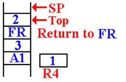
Remember our notation for return addresses: A1 for the calling routine.
FR for the return in DOFACT.

This is the status of the stack when DOFACT is first called.

The return address (A1) of the main program was pushed
first, and then the value (3) was pushed.

The value in R4, used for the return value, is not important.

It is noted that 3 > 1 so DOFACT will be called with a value
of 2. When the first recursive call is made, the stack status is
shown at left. The top of the stack has the value 2.
The return address (FR) of the DOFACT function was
first pushed, followed by the argument value.

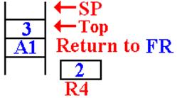
The Next Recursive Call To DOFACT

On the next call to DOFACT, the value at the top of the stack is found to be 2.

It is noted that 2 > 1.

The argument value for the next recursive call is computed,
and made ready to push on the stack.

The return address (FR) for DOFACT is pushed onto the stack.
Then the value of the new argument (1) is pushed onto the stack.

DOFACT is called again.

In this next call to DOFACT, the value at the top of the stack is
examined and found to be 1.

A return value is placed into the register R4, which has been
reserved for that use.

This is the status of the stack just before the first return.

It will return to address FRET in the function DOFACT.

The First Recursive Return

The first recursive return is to address FR (or FRET) in DOFACT.
Here is the situation just after the first recursive return.

The argument value for this invocation is
now at the top of the stack.

The value 2 is removed from the stack, multiplied
by the value in R4 (which is 1) and then stored in R4.

The return address (FR) had been popped from the
stack. The function returns to itself.

The Next Recursive Return

The next recursive return is to address FR (or FRET) in DOFACT.

Here is the situation just after the first recursive return.

Here is the status of the stack after this
return. The argument value is on the top
of the stack, followed by the return address
for the main routine.

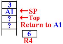On the final return, the value 3 has been removed
from the stack, multiplied by the value in R4, and
the new function value (6) is placed back into R4.

The return address (A1) has been popped from the
stack and the function returns there.

The Subroutine Linkage Problem

When a subroutine or function is called, control passes to that subroutine but must return
to the instruction immediately following the call when the subroutine exits. There are two main issues in the design
of a calling mechanism for subroutines and functions. These fall under the heading “subroutine linkage”.

1. How to pass the return address to the subroutine so that, upon completion,
it returns to the correct address. We have just discussed this problem.

2. How to pass the arguments to the subroutine and return values from it.

A function is just a subroutine that returns a value. For functions, we have one additional
issue in the linkage discussion: how to return the function value. This presentation will be a bit historical in that it will
pose a number of linkage mechanisms in increasing order of complexity and flexibility. We begin with a simple
mechanism based on early CDC–6600 FORTRAN compilers.

Pass–By–Value and Pass–By–Reference

Modern high–level language compilers support a number of mechanisms for passing
arguments to subroutines and functions. These can be mimicked by an assembler.

Two of the most common mechanisms are:

1. Pass by value, and

2. Pass by reference.

In the pass–by–value mechanism, the value of the argument is passed to the subroutine. In the pass–by–reference,
it is the address of the argument that is passed to the subroutine,
which can then modify the value and return the new value. Suppose that we want to use register R10 to pass an
argument to a subroutine. That argument is declared as follows.

FW1 DC F‘35’

The operative code would be as follows:

Pass by value: L R10,FW1 Load the value at FW1

Pass by reference: LA R10,FW1 Load the address of FW1

Returning Function Values

There is a simple solution here that is motivated by two facts.

1. The function stores its return value as its last step.

2. The first thing the calling code should do is to retrieve that value.

This simple solution is to allocate one or more registers to return function values. There seem to be no drawbacks
to this mechanism. As we have seen above, it works rather well with recursive functions. The solution used in
these lectures was to use R7 to return the value.

The CDC–6600 FORTRAN solution was to use one or two registers as needed.

CDC Nerds note that the actual register names are X6 and X7.

Argument Passing: Version 1 (Based on Early CDC–6400 FORTRAN)

Pass the arguments in the general–purpose registers. Here we use the actual names of the registers: X0 through X7.
Register X0 was not used for a reason that I cannot remember.

Registers X1 through X5 are used to pass five arguments.

Registers X6 and X7 are used to return the value of a function.

This is a very efficient mechanism for passing arguments. The problem arises when one wants more than five arguments
to be passed. There is also a severe problem in adapting this scheme to recursive subroutines. We shall not discuss this
at present for two reasons.

1. We shall meet the identical problem later, in a more general context.

2. None of the CDC machines was designed to support recursion.

Argument Passing: Version 2 (Based on Later CDC–6400 FORTRAN)

In this design, only two values are placed on the stack. Each is an address.

The return address.

The address of a memory block containing the number of arguments
and an entry (value or address) for each of the arguments.

This method allows for passing a large number of arguments.

This method can be generalized to be compatible with the modern stack–based protocols.

Example Code Based on CDC–6600 FORTRAN

Here is IBM/System 370 assembly language written in the form that the CDC FORTRAN compiler might have
emitted. Consider a function with three arguments. The call in assembly language might be.

LA R8,FRET ADDRESS OF STATEMENT TO BE
EXECUTED NEXT.

STKPUSH R8,R PLACE ADDRESS ONTO STACK

LA R8,FARGS LOAD ADDRESS OF ARGUMENT BLOCK

STKPUSH R8,R PLACE THAT ONTO THE STACK

B THEFUNC BRANCH DIRECTLY TO SUBROUTINE

A0 DC F‘3’ THE NUMBER OF ARGUMENTS

A1 DS F HOLDS THE FIRST ARGUMENT

A2 DS F HOLDS THE SECOND ARGUMENT

A3 DS F HOLDS THE THIRD ARGUMENT

FRET The instruction to be executed on return.

This cannot be used with recursive subroutines or functions.

The Solution: Use a Stack for Everything

We now turn our attention to a problem associated with writing a compiler. The specifications for the high–level language
state that recursion is to be supported, both for subroutines and functions. It is very desirable to have only one mechanism
for subroutine linkage. Some architectures, such as the VAX–11/780 did support multiple linkages, but a compiler writer
would not find that desirable. Software designers who write compilers do not like a complex assembly language; they
want simplicity.

We have a number of issues to consider:

1. How to handle the return address. This, we have discussed.

2. How to handle the arguments passed to the subroutine or function.

We have just mentioned this one.

3. How to handle the arguments and values local to the subroutine or function.

The answer is simple: put everything on the stack.

Summary of Our Approach to Recursion

Here is an approach to recursive programming that is in step with the current practice. First, we note that all recursive programming
is to be written in a high–level language; thus, the generation of the actual recursive code will be the job of a sophisticated compiler.

Consider a function call, such as Y = F1(A, B, C).

1. The compiler will generate code to push the return address onto the stack.

2. The compiler will generate code to push the arguments on the stack. Either order,
left to right or right to left is probably OK, but it must be absolutely consistent.

3. Optionally, the compiler generates code to push the argument count onto the stack.

      4.      The compiler will have a convention for use of registers to hold return values.
               This might be R4 for 16–bit and 32–bit integers, the register pair (R4, R5) for
               64–bit integers, and floating–point register 0 for real number results.

Mathematical Functions and Subroutines

We now consider a problem that occurs mostly in scientific programming and occasionally in business programming. This is the
evaluation of some of the standard functions, such as sine, cosine, logarithm, square root, etc.
There are two significant problems to be discussed.

1. The fact that the basic arithmetic instruction set of any computer includes only
the four basic operations: addition, subtraction, multiplication, and division.

2. The fact that no algorithm can be devised to produce the exact value of one of
these functions applied to an arbitrary input value.

A detailed discussion of our approach to addressing these difficulties is based on some results from Intermediate
Calculus. In this discussion, these results will only be asserted and not justified. One should study the Calculus in
order to fully appreciate our reasoning here.

Definition of an algorithm:

An algorithm is a sequence of unambiguous instructions for solving a problem.
The full definition must include the provision that the algorithm terminate for any
valid input. So we have the following definition of algorithm.

Definition: An algorithm is a finite set of instructions which, if followed, will accomplish a particular task.
In addition every algorithm must satisfy the following criteria:

      i)          input:                  there are zero or more quantities which are externally supplied;
      ii)         output:                at least one quantity is produced;
      iii)        definiteness:        each instruction must be clear and unambiguous;
      iv)        finiteness:            if we trace out the instructions of the algorithm, then for
                                             all valid cases the algorithm will terminate after a finite
                                             number of steps;
      v)         effectiveness:       every instruction must be sufficiently basic that it can in
                                             principle be carried out by a person using only a pencil and
                                             paper. It is not enough that each operation be definite as in
                                             (iii), but it must be feasible.       [page 2, R_26]

The effectiveness criterion might be restated as it being possible to map each step in the algorithm to a simple
instruction in the assembler language. In particular, only the basic steps of addition, subtraction, multiplication
and division may be used in the algorithm.

Admittedly, there are manual procedures for other processes, such as taking the square root of an integer, but
these are based on the four primitive algebraic operations.

Sample Problems

In order to illustrate a variety of system subprograms, your author has chosen the following.

1. Raising a real number to an integer power.

2. Computation of the cosine of an angle given in radian measure.

3. Computation of the square root of a non–negative real number.

In each of these cases, we shall first discuss the algorithm to be used by giving a description in a high–level
language. We then proceed to give the basis of a function, written in IBM
System 370 assembler language. As often is the case, certain necessary features related to linkage to and
from the calling program will be omitted.

Integer Exponentiation

We first consider the problem of raising a real number to an integer power. Unlike the more general problem
of raising a number to a real–number power (say X^2.817), this procedure can be completed using only the basic
operations of addition and multiplication.

The only issue to be addressed in the discussion of this problem is that of the time efficiency of the computation.
System programmers must pay particular attention to efficiency issues.

The basic problem is to take a real number A and compute F(A, N) = A^N for N ≥ 0. The simplest algorithm is easy
to describe, but not very efficient for large values of N. In terms commonly used for algorithm analysis,
this is called a “brute force” approach.

Brute Force

Function F(A, N)
     R = 1         // R = Result, what a brilliant name!
     For K = 1 to N Do
          R = R * A
     End Do
Return R

In assaying the computational complexity of this procedure, we note that the number of multiplications is a linear
function of the exponent power; specifically N multiplications are required in order to compute the N^th power of
a real number. Any competent system programmer will naturally look for a more efficient algorithm.

We now present a more time-efficient algorithm to compute F(A, N) = A^N for N ≥ 0.

This algorithm is based on representation of the power N as a binary number. Consider the computation of A¹³.
In 4-bit binary, we have 13 = 1101 = 1·8 + 1·4 + 1·2 + 1·1. What we are saying is that A¹³ = A⁸·A⁴·A²·A¹.
Our new algorithm is based on this observation.

Function F(A, N)

     R = 1
     AP = A             // AP is a to the power P
     While (N > 0) Do

          NR = N mod 2
          If NR = 1 Then R = R * AP
          AP = AP * AP
          N = N / 2     // Integer division: 1/2 = 0.

End While

Return R

One can show that the time complexity of this algorithm is log₂(N). The implementation of this algorithm in assembler
language appears simple and straightforward. The efficient implementation of this algorithm takes a bit more thought,
but not much.

In our studies of algorithm analysis and design, we identify and count the primary operations in any algorithm. Here
the key operations appear to be multiplication and division. In actual systems programming, we must pay attention to
the amount of time that each operation takes in order to execute; multiplication and division are costly in terms of time.
Can we replace either operation with a faster, but equivalent, operation?

As the multiplication involves arbitrary real numbers, there is nothing to do but pay the time cost and be happy that the
number of these operations scales as log₂(N) and not as N. But note that the division is always of a non–negative
integer by 2. Here we can be creative.

Consider the following code fragment, adapted from the algorithm above. Without changing the effect of the code,
we have rewritten it as follows.

NR = N mod 2
N = N / 2 // Integer division: 1/2 = 0.
If NR = 1 Then R = R * AP
AP = AP * AP

What we shall do in our implementation is replace the integer division by a logical right shift (double precision), using an
even–odd register pair. Let us assume that the integer power for the exponentiation is in R4, the even register of the
even–odd pair (R4, R5). Here is the code.

SR R5,R5 // Set register R5 to 0.

SRDL R4,1 // Shift right by 1 to divide by 2

CH R5,=H‘0’ // Is the old value of R4 even?

BE ISEVEN // N mod 2 was 0.

MDR F2,F4 // R = R * AP

ISEVEN MDR F4,F4 // AP = AP * AP

Let’s write a bit more of the code to see the basic idea of the algorithm. We all know that any number raised to the power 0
gives the value 1; here we say A^N = 1, if N £ 0. The only general implementation of the algorithm will use the floating–point
multiplication operator; here I arbitrarily choose the double–precision operator MDR.

Here are the specifications for the implementation.
On entry Integer register R4 contains the integer power for the exponentiation.
Floating point register 2 contains the number to be raised to the power.

On exit Floating point register 0 contains the answer.

Here is a code fragment that reflects the considerations to this point. In this code fragment, I assume that I have used the equate to set
F0 to 0, F2 to 2, F4 to 4, and F6 to 6, in the same manner in which the R symbols were equated to integer register numbers.

LD F0,=D‘0.0’ // Clear floating point register 0

CD F2,=D‘0.0’ // Is the argument zero?
BE DONE // Yes, the answer is zero.

LD F0,=D‘1.0’ // Default answer is now 1.0

LDR F4,F2 // Copy argument into FP register 4

CH R4,=H‘0’ // Is the integer power positive?

BLE DONE // No, we are done.

SR R5,R5 // Set register R5 to 0.

SRDL R4,1 // Shift right by 1 to divide by 2

CH R5,=H‘0’ // Is the old value of R4 even?

BE ISEVEN // N mod 2 was 0.

MDR F2,F4 // R = R * AP

ISEVEN MDR F4,F4 // AP = AP * AP

All we have to do now is to put this within a loop structure. Here is what we have.

POWER LD F0,=D‘0.0’ // Clear floating point register 0

CD F2,=D‘0.0’ // Is the argument zero?
BE DONE // Yes, the answer is zero.

LD F0,=D‘1.0’ // Default answer is now 1.0

LDR F4,F2 // Copy argument into FP register 4

TOP CH R4,=H‘0’ // Is the integer power positive?

BLE DONE // No, we are done.

SR R5,R5 // Set register R5 to 0.

SRDL R4,1 // Shift right by 1 to divide by 2

CH R5,=H‘0’ // Is the old value of R4 even?

BE ISEVEN // N mod 2 was 0.

MDR F2,F4 // R = R * AP

ISEVEN MDR F4,F4 // AP = AP * AP

B TOP // Go back to the top of the loop

DONE BR R14 // Return with function value.

Again, we should note that the provision for proper subroutine linkage in the above code is minimal and does not meet
established software engineering standards. All we need is a provision to save and restore the registers used in this
calculation that were not set at the call.

Before we move to consideration of the common algorithm for computing the square root of an arbitrary number, we
shall consider the more general problem of raising a number (real or integer) to an arbitrary real power. This is significantly
more difficult that that of raising a number to an integer power, or to a specific rational–number power such as ½.

Let A be an arbitrary positive number. Specifically, its value is not zero. We consider the
problem of computing F(A, X) = A^X, where X is an arbitrary real number. The general way is based on logarithms
and exponents. Because the values are more easily computed, most implementations use natural logarithms and
the corresponding exponentiation.

Let B = ln(A), the natural logarithm of A.

Then A^X = (e^B)^X = e^(BX), where e » 2.71818, is the base for the natural logarithms. Thus,
the basic parts of the general exponentiation algorithm are as follows.

1. Get rid of the obvious cases of A = 0.0 and X = 0.0.
Decide how to handle A < 0.0, as the following assumes A > 0.0.

2. Take the natural logarithm of A; call it B = ln(A).

3. Multiply that number by X, the power for the exponentiation.

      4.   Compute e^(BX), and this is the answer. Note that there is a well–known algorithm
            based on simple results from calculus to compute e to any power.
            If it makes sense, adjust for the sign of A.

The point here is that the general exponentiation problem requires invocation of two fairly complex system routines,
one to calculate the natural logarithm and one to compute the value of e^(BX). This is much slower than the computation
of an integer power. Remember that fact when writing high–level languages that require exponentiation.

Evaluating Transcendental Functions

We now discuss one standard way of computing the value of a transcendental function, given the restriction that only
the basic four mathematical operations (addition, subtraction, multiplication, and division) may be used in the
implementation of any algorithm.

This standard way consists of computing an approximation to the result of an infinite series. In effect, we sample a
moderately large number of terms from the infinite sequence, sum these terms, and arrive at a result that has acceptable
precision. As noted above, the only way to view evaluation of an infinite series as an algorithm is to state a required precision.

Here are some of the common infinite series representations of several transcendental functions. Each series can be
derived by use of a number of standard calculus techniques. The basic idea here is that of convergence, which denotes
the tendency of an infinite series to approach a limiting value, and do so more exactly as the number of terms evaluated increases.

In more precise terms, consider a function F(X) which can be represented by the infinite series
F(X) = T₀(X) + T₁(X) + T₂(X) + …. + T_N(X) + …, representing the true function value.
Define F_N(X) = T₀(X) + T₁(X) + T₂(X) + …. + T_N(X) as that value obtained by the summation of
the first (N + 1) terms of the infinite series.

A series is said to converge if for any positive number e > 0 (representing a desired accuracy), we can find an integer
N₀ such that for all N > N₀, we have |F(X) – F_N(X)| < e. There are a few equivalent ways to state this property; basically
it states that for any realistic precision, one is guaranteed that only a finite number of the terms of the infinite series must
be evaluated. For the trigonometric functions, the input must be in radians (not degrees).

SIN(X) = X – X³/3! + X⁵/5! – X⁷/7! + X⁹/9! – ….+ (–1)^N·X^2N⁺¹/(2N+1)! …

COS(X) = 1 – X²/2! + X⁴/4! – X⁶/6! + X⁸/8! – ….+ (–1)^N·X^2N/(2N)! …

EXP(Z) = 1 + Z + Z²/2! + Z³/3! + Z⁴/4! + …. + Z^N/N! + ….

LN(1+Z) = Z – Z2/2 + Z3/3 – Z4/4 + …. – (–Z)^N/N + …
Here either Z = 1 or |Z| < 1. Otherwise, the series is not useful.

Consider the problem of evaluating the sine of an angle. Here are a few of the well–known values:
SIN(0°) = 0.00, SIN(90°) = 1.00, SIN(180°) = 0.00,and SIN(–90°) = –1.00. As noted just above, the formulae are
specific to computations for angles in radians. For this reason, some systems offer trigonometric functions in pairs.
For the sine computation, we may have
SIN(q) sine of the angle, which is expressed in radians, and
SIND(q) sine of the angle, which is expressed in degrees.

Given an angle in degrees, the first thing that any computation will do is to convert the angle to equivalent radian measure.
The one exception to that would be first to translate the angle into the range –180° £ q £ 180°, by repeated additions or
subtractions of 360°. It is a well known property of all trigonometric functions that, given any integer N (positive, negative,
or 0) and angle q expressed in degrees, we have F(q) = F(q + N·360) = F(q – N·360). There may be some numerical
advantage to doing this conversion on the degree measure.

The next step, when handling an angle stated in degrees is an immediate conversion to radian measure. As 180° = p
radians, we multiply the degree measure of an angle by
(p / 180) » 0.0174 5329 2519 9432 9576 9237 to convert to radian measure.

Given an angle in radian measure, the first step would be to convert that measure into the standard range –p £ q £ p,
by repeated additions or subtractions of p. This follows the property stated above for trigonometric functions:
F(q) = F(q + 2·N·p) = F(q – 2·N·p).
The attentive reader will note that each “standard range” listed above has an overlap at its ends; basically –180° and 180°
represent the same angle, as do –p and p.

Once the angle is expressed in radians and given by a measure in the standard range, which
is –p £ q £ p, the next step in computation of the sine is to reduce the range to the more usable (–p / 2) £ q £ (p / 2)
by adapting the standard formula for SIN(X ± Y), which is
SIN(X ± Y) = SIN(X)·COS(Y) ± COS(X)·SIN(Y). The common variants are:

SIN(p/2 – q) = SIN(p/2)·COS(q) – COS(p/2)·SIN(q)
= 1·COS(q) – 0·SIN(q) = COS(q); also COS(p/2 – q) = SIN(q).

SIN(q – p/2) = SIN(q)·COS(p/2) – COS(q)·SIN(p/2)
= SIN(q)·0 – COS(q)·1 = – COS(q).

SIN(p – q) = SIN(p)·COS(q) – COS(p)·SIN(q)
= 0·COS(q) – (–1)·SIN(q) = SIN(q).

SIN(q – p) = SIN(q)·COS(p) – COS(q)·SIN(p)
= SIN(q)·(–1) – COS(q)·0 = – SIN(q)

The goal, and end result, of all of this trigonometry is to reduce the absolute value of the radian measure of the
angle to |q| < p/2. This allows an easy computation of the number of terms to be computed in the otherwise
infinite series, depending on the required accuracy.

We have: SIN(X) = X – X³/3! + X⁵/5! – X⁷/7! + X⁹/9! – ….+ (–1)^N·X^2N⁺¹/(2N+1)! …
Note that the N^th term in this series is written as T_N = (–1)^N·X^2N⁺¹/(2N+1)!. A standard result of calculus indicated
that the maximum error from terminating this series at T_N is given by
T_N = |X|^2N+1/(2N+1)!, where |X| is the absolute value of X.

Put another way, let SIN(q) represent the exact value of the sine of the angle q, represented in radians and let
S_N(q) = q – q³/3! + q⁵/5! – q⁷/7! + q⁹/9! – ….+ (–1)^N·q^2N+1/(2N+1)! represent the finite sum of the first (N + 1)
terms in the infinite series. We are guaranteed that the maximum error in using this finite sum as the sine of
the angle is given by |SIN(q) – S_N(q)| £ |X|^2N+1/(2N+1)!.

The results for our error analysis are given in the following table. Note that seven terms are all that is
required for a result to be expressed in the IBM E (Single Precision Floating Point) format, while 13 terms
are more than good enough for the IBM D (Double Precision Floating Point) format. The extended
precision floating point may require a few more terms.

N	2N + 1	(2)^2N+1	(2N+1)!	Max Error	Significant Digits
3	7	128	5040	0.025	1
5	11	2048	39,916,800	5.1307·10^–5	4
7	15	32,768	1.30767·10¹²	2.5059·10^–8	7
9	19	524,288	1.21645·10¹⁷	4.30999·10^–12	11
11	23	8,388,608	2.58520·10²²	3.24486·10^–16	15
13	27	134,217,728	1.08888·10²⁸	1.232614·10^–20	19

As an example of the fast convergence of the series, I consider the evaluation of
the cosine of 1.0 radian, about 57.3 degrees.

Look at the terms in the infinite series, written as T₀ + T₂ + T₄ + T₆ + T₈ + ...,
and construct the partial sums.

N = 0 T₀ = + 1.00000000

N = 2 X² = 1.0 T₂ = – 1 / 2 = – 0.50000000

N = 4 X⁴ = 1.0 T₄ = + 1 / 24 = + 0.04166666

N = 6 X⁶ = 1.0 T₆ = – 1 / 720 = – 0.00138889

N = 8 X⁸ = 1.0 T₈ = + 1 / 40320 = + 0.00002480

The terms are decreasing fast. How many terms do we need to evaluate to get a specified precision? Answer: Not many.

The answer for COS(1.0), after five terms in the series is 0.54030257.
My calculator computes the value as 0.540302306.

Note the agreement to six digits. Assuming that the value from my calculator is correct,
the relative error in this series sum approximation is 1.000 000 488 615, or a percentage
error of 4.89·10^–5%. After a few more terms, this result would be useable almost anywhere.

The absolute error in the above, assuming again that my calculator is correct,
is given by the difference: 0.000 000 264.
Comparison to the value 0.000 024 800, which is the maximum theoretical error,
shows that our series approximation will serve very well over a wide range of arguments.

As we have covered more than enough Assembler Language syntax to write the loop, there
is no need to write the code for this computation here. The reader may take this as an
exercise, which might actually be fun.

The structure of the computation would be a loop that sequentially builds the partial sums from the terms as
shown above. The only real question is the termination criterion for the
computation loop. There are two useable options.

      1.   Terminate after a fixed number of terms have been calculated.
            Thirteen terms should be more than adequate.
      2.   Terminate after the absolute value of the calculated term drops below a given value.