The Heritage of
the IBM System/360
Earlier Commercial Computers
Edward L.
Bosworth, Ph.D.
TSYS
Department of Computer Science
bosworth_edward@colstate.edu
Outline and
Rationale
The goal of this lecture is to
describe the early history of computing
machines manufactured by the International Business Machines Company.
I hold that many of the design
choices seen in the IBM S/370 architecture
reflect the use made of earlier computing machines, especially in 1930 – 1960.
Outline of this lecture:
1. Discussion
of technologies and computer generations.
2. Early
mechanical and electro–mechanical computers.
3. Early
electronic computing machines.
4. The
genesis of the IBM System/360: its immediate predecessors.
5. Design
choices in the IBM System/360 and System/370.
The Classic
Division by Generation
Here is
the standard definition of computer generations.
Note
that it ignores all work before 1945.
1. The
first generation (1945 – 1958) is that of vacuum tubes.
2. The
second generation (1958 – 1966) is that of discrete transistors.
3. The
third generation (1966 – 1972) is that of small-scale and
medium-scale integrated circuits.
4. The
fourth generation (1972 – 1978) is that of large–scale
and very–large–scale integrated
circuits; called “LSI” and “VLSI”.
5. The
term “fifth generation” has been widely used to describe a
variety of devices. It still has no standard definition.
Early
Computing Machines Were Mechanical
Here is
an unexpected example: the Jacquard Loom.
Though not
a
computer, it was powered by steam and controlled by punched cards.
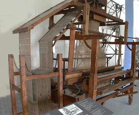
A Reconstructed Jacquard Loom
in the
Scheutz’s
Difference Engine
This is
an example of a purely mechanical computing machine.
Note the
gears and the hand crank.
Electro–Mechanical
Computing Machines
Beginning
in about 1900, the computing machines used electro–mechanical
relays. Below is a diagram of such a
relay.
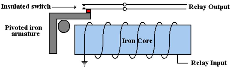
This is
an electrically activated switch.
When the
relay input is energized, the electromagnet is energized, and the
pivoted armature is moved. This causes
the switch to close.
The
Hollerith Type–III Tabulator
This
electro–mechanical computing machine dates from 1932.
Note the plug–board with wires. These were used to program the machine.
The
IBM 405: IBM's High–End Tabulator
It was first one to be called an Accounting Machine.
It was programmed by a removable plug–board with over
1600 functionally significant "hubs", with access to up to 16
accumulators.
The machine could tabulate at a rate of 150 cards per
minute, or tabulate and print at 80 cards per minute.
A
More Modern Plug–Board
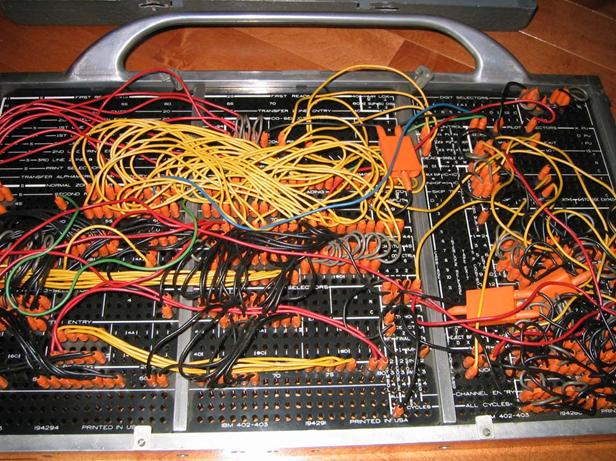
This is a plug–board from the IBM 405, manufactured
about 1946.
The
Printer for the IBM 402 (1950)
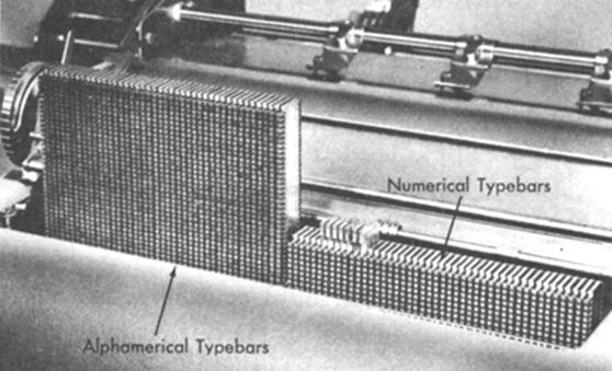
Note
that the typebars on the right can print only numerical characters.
All–Electronic
Computing Machine
These
were built with vacuum tubes, which only became sufficiently reliable in
the 1940’s. Even then, it was common for
the machine to run for only 4 hours.
Here are
four vacuum tubes from my private collection.
The
ENIAC (1945)
The
ENIAC was possible only after the problem of vacuum tube reliability
had been solved. There was also the
problem of rodents eating the wiring.
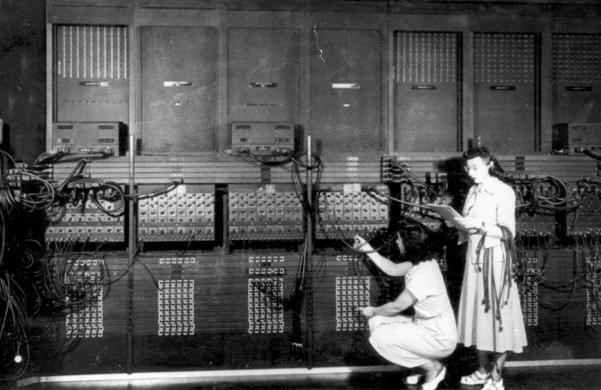
Two women
programming the ENIAC (Miss Gloria Ruth
Gorden
on the left and Mrs. Ester Gertson on
the right)
The
IBM NORC (1954)
Here is
a picture of a typical large computer of the early 1950’s.
Note the
trays of vacuum tubes in the background.
These form the computer.
The
IBM 650 (Circa 1955)
This
computer used vacuum tube technology.
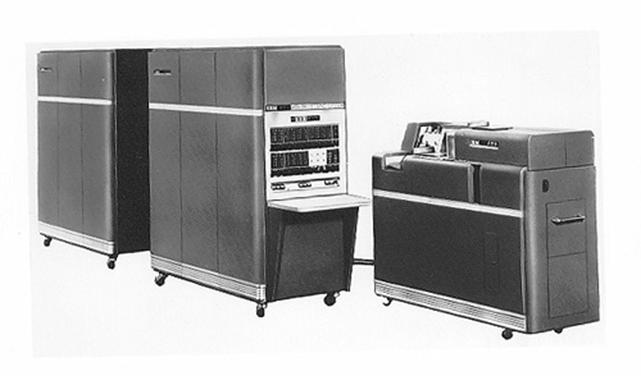
The IBM 650
– Power Supply, Main Unit, and Read-Punch Unit
Source: Columbia University [R41]
A
Block of Vacuum Tubes from the IBM 701
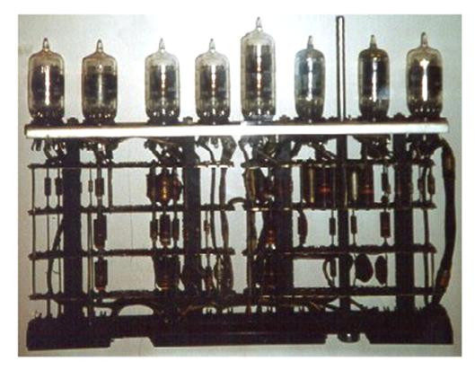
The IBM 701, produced in 1952, used replaceable
components
to facilitate maintenance.
Smaller
Components:
Transistors and Integrated Circuits
Here is
a picture showing some smaller tubes, with transistors and an
integrated circuit (presumably with a few thousand transistors).
Discrete
Transistors
In the
1960’s, computers were fabricated from circuit boards populated with
discrete transistors. Again, this
allowed for module replacement.
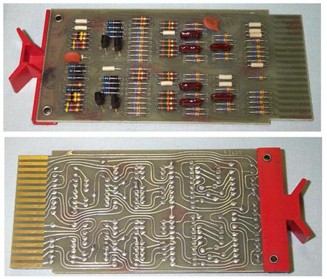
These were manufactured by the Digital Equipment
Corporation.
The “black hats” are the transistors.
Circuit
Boards Plugged Into a Backplane
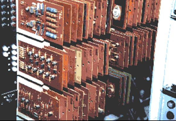
Figure: A Rack of Circuit Cards from the Z–23 Computer
(1961)
An
IBM Engineer with Three Generations of Components
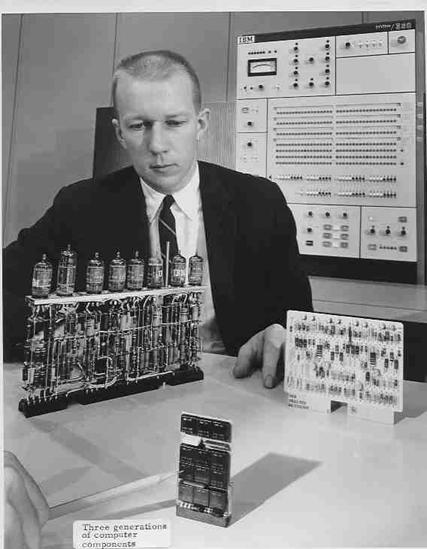
The
first generation tube component is one that we have already seen.
The
second generation discrete transistor board is a bit out of focus.
Presumably it has the same function.
Note the
pencil pointing to one of nine integrated circuits on the 3rd
generation component. Presumably, it
also has the same function as the first board.
Note
also the coat and tie. This was the IBM
corporate culture.
The IBM
S/360 might be considered an early 3rd generation computer.
Some
Line Printers
Line
printers were used to print large volume outputs, typical of a data center.
Here are two such printers, the IBM 716 and the IBM 1403.
IBM
716 IBM
1403
A
Typical “IBM Shop” of the 1960’s
Seen here (at left) is an IBM 523 gang
summary punch, which could process 100 cards a minute and (in the middle) an
IBM 82 high-speed sorter, which could process 650 punched cards a minute.
Early
IBM Product Lines
In 1960,
IBM had four major “lines” of computers:
1) the
IBM 650 line – a small, general purpose computer.
2) the
IBM 701 line, for scientific computations.
This had hardware for floating–point arithmetic, but not packed
decimal.
This includes the IBM 701, 704, 709,
7090, and 7094.
3) IBM
702 line, for commercial computations.
This had hardware for packed
decimal arithmetic, but not floating–point.
This includes the IBM 702, 705, and
7080.
4) the
IBM 7030 (Stretch).
This was a research computer. It was not produced in volume.
The big
issue is that none of these computer lines were compatible, either in
the software sense or hardware sense.
Field technicians generally were trained for the 701
line or 702 line, but not both
The IBM S/360 “Family Tree”
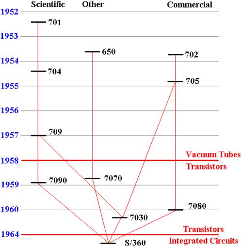
This shows the chronological “descent” of the IBM
S/360.
Some Design Goals for the System/360
Here are a number of goals for the system.
1. To replace a number of very successful, but
incompatible, computer
lines with a single computer
family.
2. To provide “an expandable system that would
serve every data processing
need”. It was to excel at all “360 degrees of data processing”.
[R11, p 11]
3. To provide a “strictly program compatible”
family of processors,
which would “ensure that the
user’s expanding needs be easily
accommodated by any model [in the
System/360 family]”.
The
System/360 was announced on April 7, 1964.
The first offerings included Models 30, 40, 50, 60,
62, and 70 [R49].
The first three began shipping in mid–1965, and the
last three were replaced by the Model 65 (shipped in November 1965) and Model
75 (January 1966).
Strict Program Compatibility
IBM
issued a precise definition for its goal that all models in the S/360
family be “strictly program compatible” [R10, page 19].
A family
of computers is defined to be strictly program compatible if and
only if a valid program that runs on one model will run on any model.
There
are a few restrictions on this definition.
1. The
program must be valid. “Invalid
programs, i.e., those which
violate the programming manual,
are not constrained to yield
the same results on all models”.
2. The
program cannot require more primary memory storage or types of
I/O devices not available on the
target model.
3. The
logic of the program cannot depend on the time it takes to execute.
The smaller models are slower
than the bigger models in the family.
“Programs dependent on execution–time will operate
compatibly if the dependence is explicit, and, for example,
if completion of an I/O operation or the timer are tested”.
The Term “Architecture”
The
introduction of the IBM System/360 produced the creation and
definition of the term “computer
architecture”.
According
to IBM [R10]
“The term architecture is used here to
describe the attributes of a system
as seen by the programmer,, i.e., the conceptual structure and functional
behavior, as distinct from the organization of the data flow and controls,
the logical design, and the physical implementation.”
The IBM
engineers realized that “logical structure (as seen by the programmer) and
physical structure (as seen by the engineer) are quite different. Thus, each may see registers, counters, etc.,
that to the other are not at all real entities.”
We shall
see in another lecture that any specific logical structure may be
supported by a number of physical implementations.
References
NOTE: The reference numbers in this set of slides
are those from the
original textbook. For that reason, they are out of order.
R_11 Mark D. Hill, Norman P. Jouppi, &
Gurindar S. Sohi, Readings in Computer
Architecture, Morgan
Kaufmann Publishers, 2000, ISBN 1 – 55860 – 539 – 8.
R_10 G. M. Amdahl, G. A. Blaauw, & F. P.
Brooks, Architecture of the IBM
System/360, IBM Journal of
Research and Development, April 1964.
Reprinted in R_11.
R_12 D. W.
Model 91: Machine
Philosophy and Instruction–Handling,
IBM Journal of Research and
Development, January 1967. Reprinted in
R_11.
R46 C. J. Bashe, W. Buchholz, et. al., The
Architecture of IBM’s Early
Computers, IBM J. Research
& Development, Vol. 25(5),
pages 363 – 376, September 1981.
Web Sites of Interest