The MARIE

Machine Architecture that is Really Intuitive and Easy.

We now define the ISA (Instruction Set Architecture) of the MARIE. This forms
the “functional specifications” for the CPU. Basic specifications of the MARIE

1. Sixteen bit words.

2. Binary, two’s–complement arithmetic. Integer range –32,768 to 32,767.

3. Stored–program computer with fixed word length and fixed instruction length.

4. 4,096 (2¹²) words of word–addressable memory. The MAR has 12 bits.
Memory addresses range from 0 through 4,095 inclusive.

5. Sixteen–bit instructions, with 4–bit opcodes and 12–bit optional addresses.
This implies a maximum of 2⁴ = 16 opcodes.

6. Two dedicated 8–bit I/O registers: InREG and OutREG.

InREG is a “magic source” of data, which are provided by some external device.
OutREG is a “magic sink” for data, which are sent to an appropriate output device.

7. A single accumulator to store temporary results. It is called “AC”, although
I shall probably slip up and call it “ACC”.

The MARIE Architecture

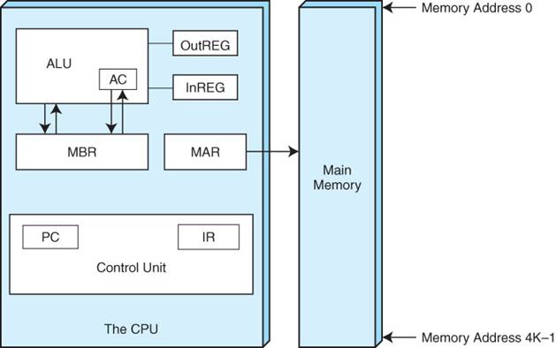
The MARIE has a 12–bit address space and a 16–bit addressable memory, so
it supports 2¹² words of memory. This is 4K words, addressed 0 to 4,095 inclusive.
It might be said to have 8 KB of memory, but it does not support byte addressing.

Note: If the MARIE has a 12–bit address space, the MAR is a 12–bit register.

The MARIE Datapath

The MARIE datapath is a bit unusual in that it has a number of direct paths into
each of the AC (accumulator) and ALU. This bus is internal to the CPU.

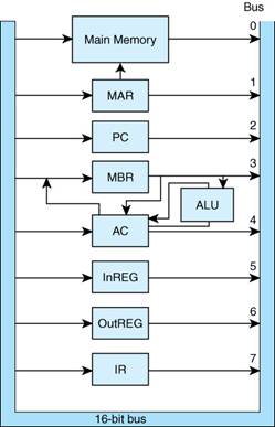
Note the direct paths MBR ® AC and MBR ® ALU. This is an artifact of the
use of a single bus internal to the CPU.

An Alternate Datapath for MARIE

As the textbook mentions, there is another datapath design that increases the CPU
efficiency at little additional complexity. Here is a small part of that datapath.

In this three–bus structure, each of the AC and MBR can be connected to an ALU
input during the same clock cycle. The output from the ALU can be made available
to either the ALU or the MBR at the end of that cycle.

We mention this just to be complete, as we shall not consider it further.

The MARIE Instruction Format

As noted above, the MARIE has a fixed word length and fixed instruction length.

Each instruction is a 16–bit word with a 4–bit opcode and 12–bit address.

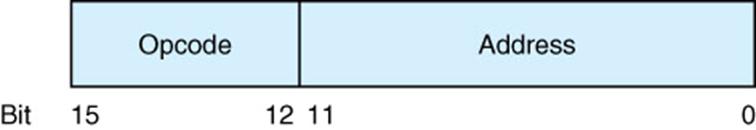
Note the allocation of 12 bits to the address.

The address in a computer is read as an unsigned binary integer. For an N–bit
representation, the unsigned integers can range from 0 through 2^N – 1.

The 12–bit unsigned integer range is 0 through 2¹² – 1 or 0 through 4,095.

Note that this is not the same as the range for a 12–bit integer in two’s–complement
representation. That range would be –2,048 through 2,047.

A Notational Problem

Consider the high–level assignment statement Y = X.

Interpretation: Take the value at the address associated with the variable X.
Place that value in the address associated with the variable Y.

In courses on Computer Architecture and Assembly Language, the notation that
appears to reference variables often specifies a memory address, not its contents.

In the notation associated with control unit design (RTL – Register Transfer Language),
this might appear as follows.

MAR ¬ X // The address X is placed into the Memory Address Register
MBR ¬ M[MAR] // The contents of this address are placed into the MBR
AC ¬ MBR // The contents of the MBR are placed into the Accumulator
MAR ¬ Y // The address Y is placed into the Memory Address Register
MBR ¬ AC // The Accumulator is copied into the Memory Buffer Register
M[MAR] ¬ MBR // The data are written into memory at address Y

In this context, what appears to be a variable name is really an associated address.

In this context, what appears to be a register name refers to the contents of that register.

More on the Notation

While there is no ambiguity possible, we often place parentheses around a register
name if the register is a source of the data. This indicates that it is the contents
of the register that are being copied.

Thus we might write either:

AC ¬ MBR // The contents of the MBR are placed into the Accumulator

AC ¬ (MBR) // The contents of the MBR are placed into the Accumulator

Remember that we also have the following.

MAR ¬ X // The address X is placed into the Memory Address Register.

MAR ¬ M[X] // The contents of address X are placed into the MAR.
// X is the address of some sort of pointer.

In terms used later in this course, the first usage is called “direct addressing” and the
second usage is called “indirect addressing”.

We shall investigate three modes of addressing (Immediate, Direct, and Indirect)
a little later in this lecture.

The Common Fetch Cycle and a Definition

The PC is the Program Counter. It is a special purpose register in the CPU.

The PC contains the address of the instruction to be executed next.

Note that the Program Counter does not count anything. It just points to the next
instruction. INTEL calls this the IP or Instruction Pointer, a much better name.

The IR is the Instruction Register. It holds the binary representation of the
machine language instruction currently being executed.

A stored program computer functions by fetching instructions from the primary
memory and executing those instructions. Here is the common fetch sequence.

MAR ¬ PC // The Program Counter is copied into the MAR

MBR ¬ M[MAR] // The contents of that address are placed into the MBR

IR ¬ MBR // The instruction at that address is placed into the IR

NOTE: AC ¬ MBR // The contents of the address are data
IR ¬ MBR // The contents of the address form an instruction

How Fetch Really Works

In reality, the computer memory cannot respond quickly enough to affect the above
fetch sequence. One must have one cycle during which memory is not accessed.

MAR ¬ PC // The Program Counter is copied into the MAR

WAIT // Wait for the memory to produce its results.

MBR ¬ M[MAR] // The contents of that address are placed into the MBR

IR ¬ MBR // The instruction at that address is placed into the IR

I hate to waste time! What can be done during this WAIT cycle that does not involve
memory? The answer comes from the fact that the most instruction most likely to be
executed is the one following this instruction.

MAR ¬ PC // The Program Counter is copied into the MAR

PC ¬ (PC) + 1 // Increment the PC to point to the next instruction.

MBR ¬ M[MAR] // The contents of that address are placed into the MBR

IR ¬ MBR // The instruction to be executed now is in the IR.
// The address of the next instruction is in the PC.

AGAIN: When an instruction is being executed, it is the address of the next instruction
(in memory) that is in the PC.

The Basic Instruction Set

We now define the basic instruction set for the MARIE by stating each instruction and
what it does. In fancier terms, we give both the syntax and semantics of each instruction.

The next few slides use RTL to describe the effect of the execution of the instruction.

The instruction has been fetched from memory. The control unit of the CPU has
decoded that instruction, and it is time for it to be executed.

All instructions share a common Fetch–Decode sequence, not specified here, because it is
not until the instruction decoding is complete that the CPU has identified the instruction.

What we are discussing here is often called the ISA (Instruction Set Architecture) of
a computer. I view the ISA as a sort of contract between the hardware and software
developers; the hardware folk deliver a specification to which the software folk design.

In the best practice, design of an ISA is the first step in the development of a new CPU.
After the ISA has been designed and agreed to, each of the software and hardware teams
has a target to which they design.

The Modified Basic Instruction Set

We should note that the instruction set discussed in these lectures and used in the MARIE
labs is the result of modifications by Dr. Neal Rogers of Columbus State University.

Here is a summary of two of those modifications.

The HALT instruction, which had opcode 7 is assigned opcode 0.

The JNS (Jump and Store) instruction, used to call functions and subroutines, has been
assigned opcode 7.

The SUBT (subtract) instruction has been renamed SUB, but keeps its opcode.

There is very good reason to assign an opcode of 0 to the HALT instruction. We shall
explain that reason on the next slide.

Almost all computer designs allocate the 0 opcode to the HALT instruction, but this
is not a sufficient reason to make the change.

Dr. Rogers has added three instructions to the MARIE instruction set. These use
opcodes 1101 (0xD), 1110 (0xE), and 1111 (0xF). These will be discussed it turn.

Why Assign Opcode 0 to HALT?

Here is the reason. We shall give a completely valid MARIE assembly language
program (without explanation) and draw your attention to one feature.

Here is the original version of the program, written in the original instruction set
with HALT assigned an opcode of 0x07.

Address	Hexadecimal Contents	Comments
100	1104
101	3105
102	2106
103	7000	The HALT instruction
104	0023	Data
105	FFE9	Data
106	0000	Nothing. Past the program end.

When entered, this will run on the emulator without problems. But consider what
will happen if the instruction at address 103 is accidentally omitted.

The Incorrect Program (HALT is Missing)

Again, this is written in the original instruction set.

Address	Hexadecimal Contents	Comments
100	1104
101	3105
102	2106
103	0023	Data The HALT is missing
104	FFE9	Data
105	0000	Nothing. Past the program end.
106	0000

In the original instruction set, this program will continue to execute until it gets to address
105. It will then continue to execute without stopping.

This behavior causes considerable difficulty in the lab.

The solution is to assign opcode 0 to HALT. Every word that the program does not
change will be automatically set to 0000, so that the program will halt fairly soon.

In the above example, once it gets to address 105, it will halt and give strange results.
But it will halt quickly.

Basic Instruction Set Definition

We now list the instructions in the modified MARIE instruction set. Each opcode is
given in both binary and hexadecimal format.

We shall follow a logical order of explanation, which is only roughly numerical.
In particular, we explain instructions 9, 8, and 7 in that order.

0. Halt Binary opcode = 0000, hexadecimal opcode = 0x00.

The machine stops execution. Nothing is changed. All register and memory
contents are preserved and can be examined with an appropriate debugger.

1. Load X Binary opcode = 0001, hexadecimal opcode = 0x01.

// Load the contents of memory address X into the Accumulator.

MAR ¬ X // Copy the memory address X into the MAR, the Memory
// Address Register. This is the only way to address memory.

MBR ¬ M[MAR] // Read memory and copy the contents of the address into
// the Memory Buffer Register.

AC ¬ (MBR) // Copy the contents of the MBR into the Accumulator.

This is often abbreviated to AC ¬ M[X]

Basic Instruction Set Definition (Part 2)

2. Store X Binary opcode = 0010, hexadecimal opcode = 0x02.

// Store the contents of the Accumulator into memory address X

MAR ¬ X // Place the address into the MAR

MBR ¬ (AC) // Copy the accumulator into the MBR

M[MAR] ¬ (MBR) // Write the MBR contents into memory at address X

This is often abbreviated as M[X] ¬ (AC)

3. Add X Binary opcode = 0011, hexadecimal opcode = 0x03.

// Add the contents of memory address X to the Accumulator

MAR ¬ X // Place the memory address into the MAR

MBR ¬ M[MAR] // Read memory and place the contents into the MBR

AC ¬ (AC) + (MBR) // Add the contents of the AC and MBR. Place in the AC.

Basic Instruction Set Definition (Part 3)

4. Subt X Binary opcode = 0100, hexadecimal opcode = 0x04.

// Subtract the contents of memory address X from the Accumulator.

MAR ¬ X // Place the memory address into the MAR

MBR ¬ M[MAR] / / Read memory and place the contents into the MBR

AC ¬ (AC) – (MBR) // Subtract MBR contents from AC contents.
// Place result in the accumulator, AC.

5. Input Binary opcode = 0101, hexadecimal opcode = 0x05.

AC ¬ (InREG) // Copy the contents of the input register into the AC.

6. Output Binary opcode = 0110, hexadecimal opcode = 0x06.

OutREG ¬ (AC) // Copy the contents of the Accumulator into the output register

Basic Instruction Set Definition (Part 4)

9. Jump X Binary opcode = 1001, hexadecimal opcode = 0x09.

// Unconditional jump to address X

PC ¬ X // The 12–bit address X, still in the IR, are copied into the PC.
// In reality, this is PC ¬ IR[11 – 0].

The program counter (PC) stores the address of the instruction that is to be
executed next.

At the control unit level, the way to force a jump is to change the value of the
program counter.

Consider the effect of the following instruction. The addresses are given in hexadecimal.

110 Jump 202

When the instruction has been loaded from address 110, the PC is then incremented to
value 111. That is the address of what appears to be the next instruction.

The effect of the instruction is to force the value 202 into the PC.
The instruction at that address is executed next.

Basic Instruction Set Definition (Part 5)

8. Skipcond Binary opcode = 1000, hexadecimal opcode = 0x08.

Skip the next instruction if the condition on the contents of the Accumulator is met.
The three conditions are : AC < 0, AC = = 0, AC > 0.

At this point, the PC already points to the next instruction, so we skip that
instruction merely by again incrementing the PC.

This is the basic conditional branch instruction. Instructions of this type were seen
on early computers (mostly before 1960), but have not been used recently.

Remember that the instruction is held in the 16 bit Instruction Register, with bits
numbered left to right as 15 through 0. Here IR[15 – 12] = 1000.

Here is a version of the explanation.

If IR[11–10] = 00 and AC < 0, then PC ¬ (PC) + 1 // Skip next instruction.

If IR[11–10] = 01 and AC = 0, then PC ¬ (PC) + 1 // Skip next instruction.

If IR[11–10] = 10and AC > 0, then PC ¬ (PC) + 1 // Skip next instruction..

I am greatly tempted to add a condition for IR[11–10] = 11, but shall resist.

More on SkipCond

If IR[11–10] = 00, then skip the next instruction if AC < 0.

IR Bit	15	14	13	12	11	10	9	8	7	6	5	4	3	2	1	0
	1	0	0	0	0	0	0	0	0	0	0	0	0	0	0	0
	8				0				0				0

Assembled as 0x8000. Write as Skipcond 000

If IR[11–10] = 01, then skip the next instruction if AC = 0.

IR Bit	15	14	13	12	11	10	9	8	7	6	5	4	3	2	1	0
	1	0	0	0	0	1	0	0	0	0	0	0	0	0	0	0
	8				4				0				0

Assembled as 0x8400. Write as Skipcond 400

If IR[11–10] = 10, then skip the next instruction if AC > 0.

IR Bit	15	14	13	12	11	10	9	8	7	6	5	4	3	2	1	0
	1	0	0	0	1	0	0	0	0	0	0	0	0	0	0	0
	8				8				0				0

Assembled as 0x8800. Write as Skipcond 800

Still More On Skipcond

Here is a graphical depiction of the Skipcond instruction.

If the condition is true, the next instruction is skipped.
If the condition is false, the next instruction is executed.

Two common uses of the Skipcond. For example, use Skipcond 800 // Skip if AC > 0

1. Skipcond 800 // Skip next instruction if AC > 0

Halt // Halt if AC £ 0

Next Instruction // Continue here if AC > 0

2. Continue execution elsewhere if the condition is false.

Skipcond 800 // Skip next instruction if AC > 0

Jump AC_LE_0 // Go to this address if AC £ 0

Next Instruction // Continue here if AC > 0

SkipCond: Specific Example

Consider the following code sequence.

110 Skipcond 800 // Skip next if AC > 0

111 Clear

112 Store 200

As the Skipcond instruction is being executed, the PC already has the value 111,
which is the address of the next instruction.

If the value in the AC is positive, the value in the PC is incremented by 1 to
the value 112. In that case, the instruction at address 112 is executed next.

If the value in the AC is not positive, the value in the PC is not altered.
The instruction at address 111 is executed next,
followed by the instruction at address 112.

Basic Instruction Set Definition (Part 6)

7. JnS X Binary opcode = 0111, hexadecimal opcode = 0x07.

// Store the next address into address X and jump to address (X + 1).

MBR ¬ PC // Copy the program counter into the MBR

MAR ¬ X // Copy the address into the MAR

M[MAR] ¬ MBR // Store the MBR into the memory at address X.
// This places the return address at address X.

MBR ¬ X // Place the target address back into the MBR.
// This is the address itself, not the contents of the address.

AC ¬ 1 // Set the AC to the value 1

AC ¬ AC + MBR // Add the contents of the MBR to the AC

PC ¬ AC // Change the value of the PC (Program Counter)
// This forces a jump.

This is a bit tricky, so I shall given an example.

The Basic Idea of a Subroutine or Function

Consider the following code, written in the MARIE assembler language. The
instruction is found at address 120, a value chosen at random.

120 JnS Sub_1

The instruction immediately following this instruction is found at address 121.

The subroutine call has a number of steps.

1. Execute the code at the address associated with the label Sub_1.

2. Return to address 121, that of the instruction following the subroutine call,
and execute that instruction next.

At the control level, we face the problem of how to save the return address.
Modern computers use a system stack to store this address, but we must use
a more primitive mechanism.

The return address is stored at the first address of the subroutine and execution
begins at the second address associated with it. For the above, we have

Address Sub_1 is a holding spot for the return address
Address Sub_1 + 1 stores the first executable instruction of the subroutine

Sample: Function Call with Return Value in the AC

Consider the following fragments of code, where all addresses are given in hexadecimal
and most are chosen at random.

11A JnS 240 // Call the function

11B Store 322 // Store the return value

240 Hex 0 // Holding location for return address

241 Clear // First instruction of the function.

At the moment the JnS instruction is executed, the PC contains the value 0x11B,
which is the address of the instruction following it.

MBR ¬ PC // This forces the value 0x11B into the MBR.

MAR ¬ X // This forces the value 0x240 into the MAR.

M[MAR] ¬ MBR // This stores the value 0x11B into the word at address 0x240.

Sample: Function Call (Part 2)

At this point, we have the following.

11A JnS 240 // Call the function

11B Store 322 // Store the return value

240 Hex 11B // Holding location for return address

241 Clear // First instruction of the function.

MBR ¬ X // Place the target address, 0x240, back into the MBR.

AC ¬ 1 // Set the AC to the value 1

AC ¬ AC + MBR // Add the contents of the MBR to the AC.

// Now the AC contains the value 0x241.

PC ¬ AC // Change the value of the PC (Program Counter) to 0x241.
// This forces a jump.

Basic Instruction Set Definition (Part 7)

10. Clear Binary opcode = 1010, hexadecimal opcode = 0x0A.

// Clear the accumulator

AC ¬ 0.

11. AddI Binary opcode = 1011, hexadecimal opcode = 0x0B.

AC ¬ AC + M [ M[X] ] // Go to address X and get the value M[X], the value
// the value stored at address X, to be the target
// address. Add the value at that address to the AC.

MAR ¬ X // Address into the MAR

MBR ¬ M[MAR] // Read that address to get the target address

MAR ¬ MBR // Target address into the MAR

MBR ¬ M[MAR] // Get the target value

AC ¬ AC + MBR // Add to the accumulator.

Basic Instruction Set Definition (Part 8)

12. JumpI Binary opcode = 1100, hexadecimal opcode = 0x0C.

PC ¬ M[X] // Go to address X. Use the value M[X], the value stored at
// address X, as the target address for the jump.

MAR ¬ X // Get the target address into the MAR

MBR ¬ M[MAR] // Get the value at that address into the MBR

PC ¬ MBR // Force a jump to that address.

Consider now the code used to illustrate the JNS instruction. Focus on the subroutine.

240 Hex 11B // Holding location for return address

241 Clear // First instruction of the function.

More code

JumpI 240 // The return instruction.

Here, the instruction “JumpI 240” indicates that the value stored at address 240 will
be the target address for the Jump. That value is 11B.

13. LoadI Binary opcode = 1101, hexadecimal opcode = 0x0D.

// Load indirect into the accumulator.

AC ¬ M [ M[X] ] // Go to address X and get the value M[X], the value stored
// at address X, to be the target address.
// Load the value at that address into the AC.

MAR ¬ X // Address into the MAR

MBR ¬ M[MAR] // Read that address to get the target address

MAR ¬ MBR // Target address into the MAR

MBR ¬ M[MAR] // Get the target value

AC ¬ MBR // Load into the accumulator.

NOTE: The original notes of 9/23/2010 are incorrect for this instruction.
For some reason, I thought that this was “Load Immediate”. It is not.

Basic Instruction Set Definition (Part 9)

14. AddM Binary opcode = 1110, hexadecimal opcode = 0x0E.

// Add immediate to the accumulator.

AC ¬ AC + IR[11 – 0] // The 12–bit unsigned integer in bits 11 through 0
// of the Instruction Register is added to the
// value in the accumulator and stored there.

15. SubM Binary opcode = 1111, hexadecimal opcode = 0x0F.

// Subtract immediate from the accumulator.

AC ¬ AC – IR[11 – 0] // The 12–bit unsigned integer in bits 11 through 0
// of the Instruction Register is subtracted from the
// value in the accumulator and stored there.

Addressing Modes: Immediate, Direct, and Indirect

The instruction set as implemented by Dr. Rogers, has three distinct addressing modes.
We shall use the Add instructions to illustrate.

Add X AC ¬ AC + M[X] Direct mode

AddI X AC ¬ AC + M [M[X] ] Indirect mode

AddM X AC ¬ AC + X Immediate mode

Here is a very important distinction between assembly language and higher level
languages. In assembly language, the label X refers to an address and not the
contents stored at that address.

More specifically, the idea of a variable is a construct of higher level languages.
Consider the following, where the label X refers to address 200.

200 Dec 1234

In assembly language, X has the value 200, while M[X] has the value 1234.

In a higher level language (with LISP excepted), the symbol X would refer to the
value stored at address X and not to the address itself.

Addressing Modes: Example

Consider the following code fragments, where X refers to the address 200.
Suppose that the accumulator, AC, has been cleared before executing each instruction.

Sample 1: Add X // Direct addressing

Sample 2: AddI X // Indirect addressing

Sample 3: AddM X // Immediate addressing

Suppose the following memory contents
200 403 // Decimal value
403 300 // Decimal value

Sample 1: AC¬ AC + M[X]
AC ¬ AC + M[200] AC ¬ AC + 403. Now AC = 403.

Sample 2: AC¬ AC + M[M [X] ]
AC¬ AC + M[M [200] ]
AC¬ AC + M[403 ] AC ¬ AC + 300. Now AC = 300.

Sample 3: AC¬ AC + X AC¬ AC + 200. Now AC = 200.

The Utility of Immediate Mode

Consider the two fragments of code which appear to have the identical effect.

Sample 1: Add One // Add value stored at address One

One, DEC 1 // The value is decimal 1.

Sample 2: AddM 1 // Add the value 1.

The first code fragment is susceptible to a common coding problem.
Consider the following code fragment; surely this is an error.

Clear // Clear the accumulator

Add One // Add the value at label One

Add One // Now presumably the AC has value 2

Store One // Now the label One may have value 2.

One, Dec 1 // It started out with value 1, but
// now has value 2 (despite its label).

This problem actually occurred in early forms of BASIC.